Accurately representing words as vectors is a challenging, but necessary task in machine learning. Consider the following sentences:
- The garden is pretty
- The garden is beautiful
As humans we know that “pretty” and “beautiful” are similar, but how can we learn vector representations of these words so that they are “close” together? If this can be done, we can start to tackle bigger challenges, such as understanding customer reviews and summarizing content.
The goal of this post is to first explain the intuition behind these 3 methods for learning word embeddings (word2vec, GloVe, fasttext), then provide Python code to get started using them quickly.
Word2Vec
Word2vec really refers to two models for learning word vectors: the continuous bag-of-words (CBOW) and the skip-gram model. They are very similar - CBOW accepts context words as input and predicts a target word, whereas the skip-gram accepts a target word as input and predicts a context word.
Although we will primarily focus on the skip-gram, both models are single layer neural networks that accept one-hot encoded vectors as input. We learn the weights of the hidden layer, and each row of this weight matrix is a word vector. The algorithm forces word vectors closer to each other every time words appear in each other’s context, regardless of position in the context window. It does this by: (1) maximizing the probability that an observed word appears in the context of a target word and (2) minimizing the probability that a randomly selected word from the vocabulary appears in the context of the target word.
If your understanding of neural network weights and the weight matricies is still shakey, this chapter gives a good into.
Deep Dive
The main idea behind the skip-gram model is that we take a word in an input sequence as the target word, and predict its context words. The context of a word is the $m$ words surrounding it. In figure 1, the window size is 2, the target word (“into”) is in red and its context words (“problems”, “turning”, “banking”, “crises”) are in blue.
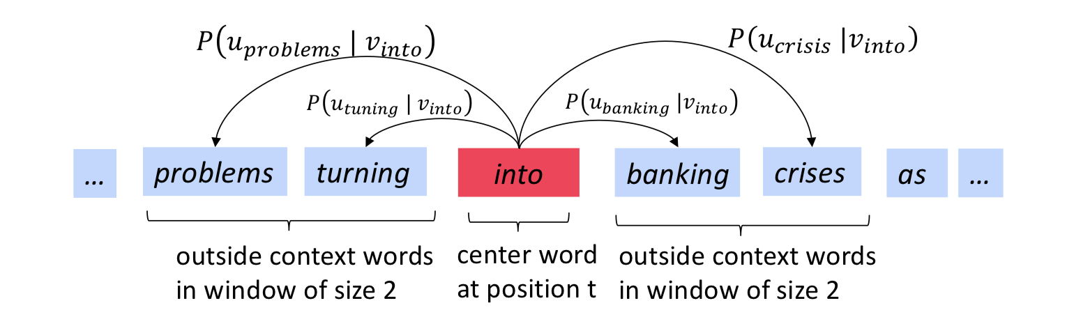
Figure 1: The skip gram prediction of target word “into” with window size 2. Taken from Stanford’s NLP course
Let’s formalize some notation. We have an input sequence of words, $w_1, w_2,.., w_T$, each of which has a context window, $-m \le j \le m$. We’ll call this input sequence the corpus, and all its unique words the vocabulary. Each word in the vocabulary will have 2 vector representations during training, $u_o$ when it’s a context word and $v_c$ when it’s a target word. In figure 1, $u_{turning}$ is the vector representation of “turning” as a context word, and $v_{banking}$ is the vector representation of “banking” as a target word.
We want to calculate the probability that each word in the window, $w_{t+j}$, appears in the context of the target word $w_t$. We’ll refer to this probability as $p(w_{t+j} \lvert w_t; \theta)$. This may seem weird, but the probability is based on the vector representations of each word. When we encounter a word in the context of another, we alter their vector representations to be “closer”. So the more we see words in each other’s context, the closer their vectors are. The function $J(\theta)$ below describes this; $\theta$ is a placeholder representing all the vector representations. We minimize $-J(\theta)$ in order to find the optimal parameters that will maximize $p(w_{t+j} \lvert w_t; \theta)$.
\[J(\theta) = -\frac{1}{T} \sum^{T}_{t = 1} \sum_{-m \le j \le m, j \ne 0} log(p(w_{t+j} \lvert w_t; \theta))\]The only problem here is we have no idea how to find $p(w_{t+j} \lvert w_t; \theta)$. We’ll start with using the softmax function. This essentially calculates how similar a context word, $u_o$, is to target word $v_c$, relative to all other context words in the vocabulary. The measure of similarity between two words is measured by the dot product $u_o^T v_c$, and a larger dot product means more similar words.
\[p(w_{t+j} \lvert w_t; \theta) = \frac{e^{u_o^T v_c}}{\sum_{w=1}^W e^{u_w^T v_c}}\]Where:
- $W$ is the size of the vocabulary
- $c$ and $o$ are indices of the words in the vocabulary at sequence positions $t$ and $j$ respectively
- $u_o = word2vec(w_{t+j})$
- $v_c = word2vec(w_t)$
Although we now have a way of quantifying the probability a word appears in the context of another, the $\sum_{w=1}^W e^{u_w^T v_c}$ term requires us to iterate over all words in the vocabulary, making it computationally inefficient. To deal with this, we must approximate the softmax probability. One way of doing this is called negative sampling.
Negative Sampling Loss
Negative sampling overcomes the need to iterate over all words in the vocabulary to compute the softmax by sub-sampling the vocabulary. We sample $k$ words and determine the probability that these words do not co-occur with the target word. The intuition behind this is that a good model should be able to differentiate between data and noise.
To incorporate negative sampling, the objective function needs to be altered by replacing $p(w_{t+j} \lvert w_t)$ with:
\[log(\sigma(u_o^T v_c)) + \sum_{i = 1}^{k}E_{j \sim P(w)} [log(\sigma(-u_j^T v_c))]\]Where $\sigma(.)$ is the sigmoid function.
The new objective function becomes:
\[J(\theta) = \frac{-1}{T} \sum_{t=1}^{T}J_t(\theta) \notag\] \[J_t(\theta) = log(\sigma(u_o^T v_c)) + \sum_{i = 1}^{k}E_{j \sim P(w)} [log(\sigma(-u_j^T v_c))] \notag\] \[P(w) = U(w)^{3/4}/Z \notag\]Let’s look at each component of and try to convince ourselves this makes sense.
The first part, $log(\sigma(u_o^Tv_c))$, can be interpreted as the log probability of the target and context words co-occurring. We want the model to find $u_o$ and $v_c$ to maximize this probability.
The second part, $\sum_{i = 1}^{k}E_{j \sim P(w)} [log(\sigma(-u_j^T v_c))]$, is where the negative sampling happens. Let’s break this up more to make it clearer. It’ll come in handy to note that $\sigma(-x) = 1 - \sigma(x)$.
We can first drop the $E_{j \sim P(w)}$ term, since we already know we will be sampling words from some distribution, $P(w)$. We end up with:
\[\sum_{i = 1}^{k} log(\sigma(-u_j^T v_c)) = \sum_{i = 1}^{k} log(1 - \sigma(u_j^T v_c)) \notag\]Now that this is easier to read, we’re taking the log of 1 minus the probability that the sampled word, $j$, appears in the context of the target word $c$. This is just log probability that $j$ does not appear in the context of the $c$. Since $j$ is randomly drawn out of ~$10^6$ words, there’s a very small chance it appears in the context of $c$, so this probability should be high. We do this for each of the $k$ sampled words.
Finally, we have to specify a distribution for negative sampling, $P(w) = U(w)^{3/4}/Z$. Here, $U(w)$ is the count of each word in the corpus (unigram distribution) and is raised to the $\frac{3}{4}$th power to sample rarer words in the vocabulary. $Z$ is just a normalization term to turn $P(w)$ into a probability distribution.
To summarize, this loss function is trying to maximize the probability that word $o$ appears in the context of word $c$, while minimizing the probability that a randomly selected word from the vocabulary does not appear in the context of word $c$. We use the gradient of this loss function to iteratively update the word vectors, $u_o$ and $v_c$, and eventually get our word embeddings.
Here is a great tutorial on the skip-gram model!
GloVe
GloVe (Global Vectors) is another architecture for learning word embeddings that improves on the skip-gram model by incorporating corpus statistics. Since the skip-gram model looks at each window independently, it loses corpus statistics. In contrast, GloVe uses word co-occurrence counts to capture global information about the corpus. GloVe learns word embeddings by minimizing the difference between word vector dot products and their log co-occurrence counts.
Deep Dive
The Co-Occurrence Matrix
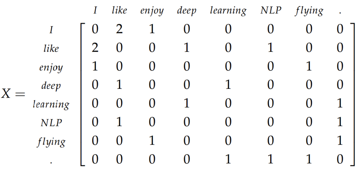
The co-occurrence matrix, $X$, is generated from the corpus and vocabulary. The entry at $X_{ij}$ is then the number of times word $j$ occurs in the context of word $i$. Context is defined in the same way as the skip-gram model. Summing over all the values in row $i$, will give the number of words that occur in its context, $X_i = \sum_k X_{ik}$. Then the probability of word $j$ occurring in the context of word $i$ is $P(i \lvert j) = \frac{X_{ij}}{X_i}$.
Below is the co-occurrence matrix for the corpus containing:
- “I like deep learning.”
- “I like NLP.”
- “I enjoy flying.”
From Softmax to GloVe
We can find global loss using the softmax function, $Q_{ij}$, by summing over all target-context word pairs.
\[J = - \sum_{i \in corpus} \sum_{j \in context} log (Q_{ij}) \notag\]Since words $i$ and $j$ appear $X_{ij}$ times in the corpus, we don’t need to iterate over all windows in the corpus, but can iterate over the vocabulary and multiply by the co-occurrence count.
\[J = - \sum_{i = 1}^{W} \sum_{j = 1}^{W} X_{ij} log Q_{ij} \notag\]Re-arranging some terms, we can come up with this:
\[J = - \sum_{i = 1}^{W} X_{i} \sum_{j = 1}^{W} P_{ij}log(Q_{ij}) \notag\]
What’s going on here?
- Where did $P_{ij}$ come from? - Remember that $P_{ij} = \frac{X_{ij}}{X_i}$ and $X_i = \sum_k X_{ik}$, therefore we can substitute $X_{ij} = P_{ij}X_i$.
- What’s the relationship between $P_{ij}$ and $Q_{ij}$? - $P_{ij}$ is the probability that word $j$ appears in the context of word $i$, but $Q_{ij}$ is also the probability that word $j$ appears in the context of word $i$. The difference between the two lies in how they are calculated. $P_{ij}$ is calculated using the co-occurrence matrix and doesn’t change. $Q_{ij}$ is the naive softmax probability, that is calculated using the dot product of word vectors $u_j$ and $v_i$. We have the ability to change $Q_{ij}$ by changing these vectors.
- What’s the point of $P_{ij}log(Q_{ij})$? - Now that we’ve refreshed our memory of $P$ and $Q$, we can see that $P$ is the true probability distribution of context and target words, and $Q$ is some made up distribution based on the “goodness” of the word vectors. We really want these two distributions to be close to each other. Observing $H = P_{ij}log(Q_{ij})$, when $P$ and $Q$ are close to each other, $H$ is small, and when $P$ and $Q$ are far apart, $H$ is larger. Our end goal is the minimization of $J$, so the smaller $H$ is the better. This term is the cross-entropy between distributions $P$ and $Q$.
The problem here is that cross-entropy requires normalized versions of $Q_{ij}$ and $P_{ij}$ which we have to iterate over the entire vocabulary to calculate. This is the reason for using Negative Sampling in the skip-gram model. GloVe’s approach to this is dropping the normalization terms completely, so we end up with $\hat{P}$ and $\hat{Q}$, which are unnormalized distributions. The cross-entropy function is now useless, so we change our objective function to be a squared error function.
\[\hat{J} = \sum_{i = 1}^{W} X_{i} \sum_{j = 1}^{W} (\hat{P}_{ij} - \hat{Q}_{ij})^2 \notag\]Now we have the squared error, weighted by the number of co-occurrences of words $i$ and $j$. There’s one last problem with this, which is that some co-occurrence counts can be massive. This will affect both the weights, $X_i$, and $\hat{P_{ij}} = X_{ij}$. To deal with this explosion in the squared term, we take $log(hat{P})$ and $log(hat{Q})$) and to deal with the explosion of weights, we introduce a function, $f$ that caps the co-occurrence count weight. We’ll apply $f$ to each target-context pair, $X_{ij}$ as opposed to only $X_i$. The new loss function becomes:
\[\hat{J} = \sum_{w = 1}^{W} \sum_{w = 1}^{W} f(X_{ij}) (u_j^T v_i - log(X_{ij}))^2 \notag\]This is the loss function that the GloVe model minimizes.
Fasttext
Fasttext is a powerful library for learning word embeddings that was introduced by Facebook in 2016. Its roots come from the word2vec models.
Word2vec trains a unique vector for each word, ignoring important word sub-structure (morphological structure) and making out-of-vocabulary prediction impossible. Fasttext attempts to solve this by treating each word as a sum of its subwords. These subwords can be defined in any way, however the simplest form is a character n-gram. A vector representation is associated with each n-gram, then the vector for each word is simply the sum of each of its n-grams. Fasttext learns word embeddings for each subword, then treats each word as a sum of its subwords.
Deep Dive
Before starting, we’ll take a step back to quantifying how similar two word vectors are. Both GloVe and word2vec do this using dot products, however we can think of the similarity more generally as an arbitrary function, $s(u_j, v_c)$.
Fasttext redefines this similarity measure, and represents words as a sum of smaller words, each of length $n$, called n-grams. To help the model learn prefixes and suffixes, we append “<” to the front and “>” to the back of each word. Then for n=3, the n-grams of “where” are:
<where> = [<wh, whe, her, ere, re>]
We have no way of determining the difference between the subword “her” and the full-word “her” (there definitely should be a difference). Appending the special characters around each word helps with this, as the tri-gram “her” is now different from the sequence “<her>”.
More formally, suppose we have all n-grams in the vocabulary, $G$, each represented by a vector, $\boldsymbol{z}_g$. We can refer to all the n-grams of some word, $w$, by $G_w$. Then $w$ can be represented as a sum of all n-grams. The new similarity function becomes:
\[s(w, c) = \sum_{g \in G_w} \boldsymbol{z}_g^T v_c \notag\]We learn the embeddings of each character n-gram and then each word embedding is a sum of its n-gram vectors.
Word Embeddings in Python
Now let’s explore word embeddings using pre-trained models in the gensim Python package. If you don’t have it installed, run pip install gensim in your command line. Gensim offers pre-trained models from their gensim.downloader method and each model used here embeds words in a 300-dimensional space. A full list of the models available can be found here, or by running python -m gensim.downloader --info in your command line.
import gensim
import gensim.downloader as api

from sklearn.decomposition import PCA
import matplotlib.pyplot as plt

# clearer images if you're using a Jupyter notebook
%config InlineBackend.figure_format='retina'
Word2vec
For word2vec, we’ll use Google’s News dataset model, trained on news articles with a vocabulary of 3 million words and 300 dimensional embedding vectors. This repo has an in-depth analysis of the words in the model.
word2vec_model_path = "word2vec-google-news-300"
print(api.info(word2vec_model_path))

word2vec_model = api.load(word2vec_model_path)
w2v = word2vec_model.wv

# remove from env
del word2vec_model
GloVe
The glove-wiki-gigaword-300 model used here is trained on 6B tokens from Wikipedia 2014 and the Gigaword dataset, other pre-trained GloVe models can be downloaded from Stanford or from Gensim.
glove_model_path = "glove-wiki-gigaword-300"
print(api.info(glove_model_path))

glove_model = api.load(glove_model_path)
glove = glove_model.wv

del glove_model
Fasttext
Fasttext provides pre-trained models on for multiple languages, which can be used in different ways (through the command line, downloading the model, through gensim, etc.). We’ll use the English model provided by Gensim which is trained on Wikipedia 2017 and news data, but you can go through their Github to see more.
Word Comparison
Now we have vector representations for all words in the vocabulary in wv and can compare the different models. We’ll add and subtract some word vectors, then see what the closest word to the resulting vector is. Papers and blog posts have exhausted the “king” - “man” + “woman” = “queen” example, so I’ll present some new ones.
Results generated by the find_most_similar function are of the form (word, cosine similarity), where each word is the closest to the one parsed into the function. Cosine similarity values closer to 1 mean that the vectors (words) are more similar. The function definition can be found in the Appendix.
Start with: doctor - man + woman
print ("word2vec: Doctor - Man + Woman")
find_most_similar(w2v["doctor"] - w2v["man"] + w2v["woman"], w2v,
                  ["man", "doctor", "woman"])

print ("GloVe: Doctor - Man + Woman")
find_most_similar(glove["doctor"] - glove["man"] + glove["woman"], glove,
                  ["man", "doctor", "woman"])

print ("fasttext: Doctor - Man + Woman")
find_most_similar(fasttext["doctor"] - fasttext["man"] + fasttext["woman"], fasttext,
                  ["man", "doctor", "woman"])
 word2vec: Doctor - Man + Woman
 [('gynecologist', 0.7276507616043091),
  ('nurse', 0.6698512434959412),
  ('physician', 0.6674120426177979)]

 GloVe: Doctor - Man + Woman
 [('physician', 0.6203880906105042),
  ('nurse', 0.6161285638809204),
  ('doctors', 0.6017279624938965)]

 fasttext: Doctor - Man + Woman
 [('gynecologist', 0.6874127388000488),
  ('nurse-midwife', 0.6773605346679688),
  ('physician', 0.6561880111694336)]
Interesting, what about if we make a subtle change to doctor - woman + man?
print ("word2vec: Doctor - Woman + Man")
find_most_similar(w2v["doctor"] - w2v["woman"] + w2v["man"], w2v,
                  ["man", "doctors", "doctor", "woman"])

print ("GloVe: Doctor - Woman + Man")
find_most_similar(glove["doctor"] - glove["woman"] + glove["man"], glove,
                  ["man", "doctors", "doctor", "woman", "dr."])

print ("fasttext: Doctor - Woman + Man")
find_most_similar(fasttext["doctor"] - fasttext["woman"] + fasttext["man"], fasttext,
                  ["man", "doctors", "doctor", "woman", "dr."])
word2vec: Doctor - Woman + Man
[('physician', 0.6823904514312744),
 ('surgeon', 0.5908077359199524),
 ('dentist', 0.570309042930603)]

GloVe: Doctor - Woman + Man
[('physician', 0.5128607153892517),
 ('he', 0.4661550223827362),
 ('brother', 0.46356332302093506)]

fasttext: Doctor - Woman + Man
[('physician', 0.6969557404518127),
 ('docter', 0.6826808452606201),
 ('non-doctor', 0.6698156595230103)]
This is a different result from the original results. Biases in the training data are expressed by the model. Also interestingly, there are some misspelled words in fasttext. This is because of the difference in learning methods.
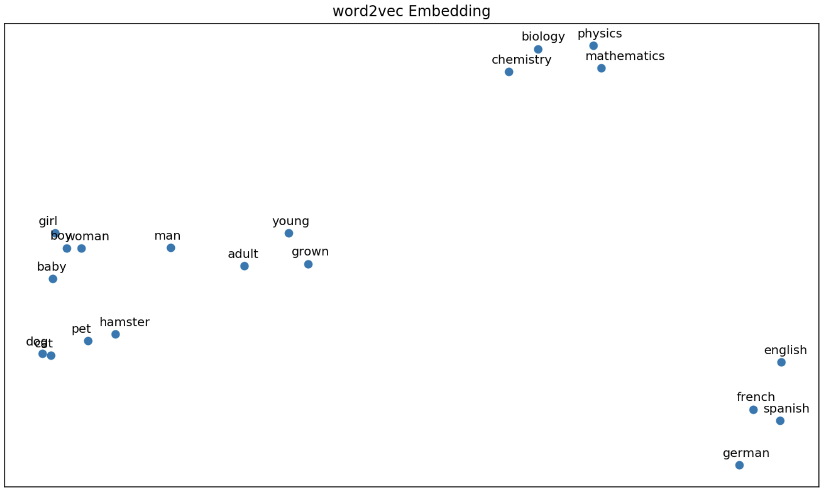
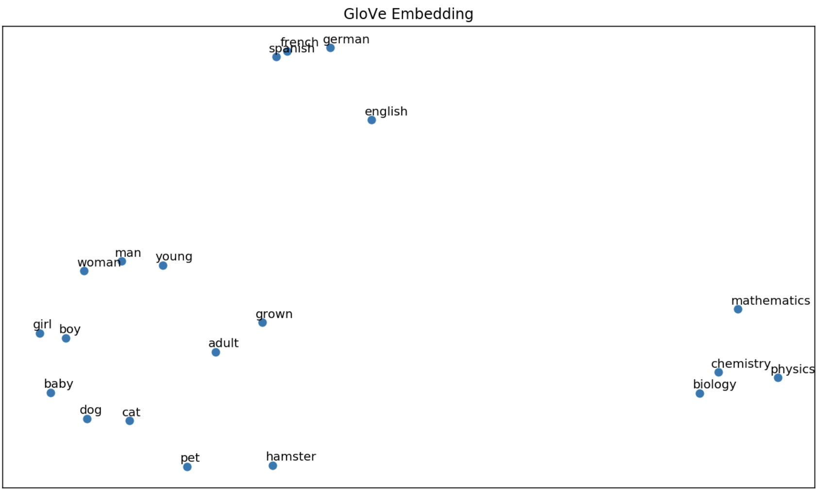
Visualizing Embeddings
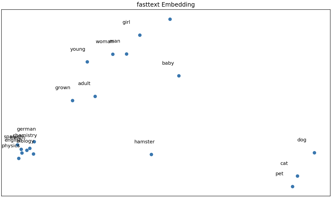
For the sake of completeness, I plotted words from different walks of life to see if the algorithms were able to unravel their semantic similarities/differences. The first 2 principal components of each word vector are plotted. Some expected similarities are seen here, however, we lose a lot of information from reducing the dimension from 300 to 2.
plot_embeds(["dog", "cat", "hamster", "pet"] +                   # animals
            ["boy", "girl", "man", "woman"] +                    # humans
            ["grown", "adult", "young", "baby"] +                # age
            ["german", "english", "spanish", "french"] +         # languages
            ["mathematics", "physics", "biology", "chemistry"],  # natural sciences
            w2v,
            title = "word2vec Embedding")
# run this again, but changing w2v to glove and fasttext
Wrapping up, there are some key differences between word2vec (skip-gram), GloVe and fasttext. The skip-gram iterates over the corpus predicting context words given a target word. GloVe builds on this by incorporating global corpus statistics using word co-occurrences. The results are similar to word2vec. Fasttext also builds on word2vec by breaking each word into a sum of its sub-words. It learns vectors for each subword, then combines them for prediction. This allows out-of-vocabulary prediction, but introduces the risk of misspelled words.
Both word2vec and GloVe can be used as frameworks for learning general similarities in text without considering what each token is made of. This makes them useful for tasks like finding similar movies given a sequence of movies watched by users. Fasttext on the other hand is more robust for translation tasks, where the likelihood of encountering an out-of-vocabulary word is higher.
More Code
# find the 3 most similar words to the vector "vec"
def plot_embeds(word_list, wv, title = None, word_embeddings = None, figsize = (12,7)) :
    # pca on the embedding
    pca = PCA(n_components=2)
    X = pca.fit_transform(wv[word_list])

    ax = plt.figure(figsize=figsize)
    ax.subplots()
    _ = plt.scatter(X[:,0], X[:,1])
    for label, point in list(zip(word_list, X)):
        _ = plt.annotate(label, (point[0] - 0.075, point[1] + 0.075))
    # Turn off tick labels
    plt.title(title)
    plt.xticks([])
    plt.yticks([])

def find_most_similar (vec, wv, words = None) :
    # vec: resulting vector from word Arithmetic
    # words: list of words that comprise vec
    s = wv.similar_by_vector(vec, topn = 10)
    # filter out words like "king" and "man", or else they will be included in the similarity
    if (words != None) :
        word_sim = list(filter(lambda x: (x[0] not in words), s))[:3]
    else :
        return (s[:3])
    return (word_sim)