Ordinary VS Bayesian Linear Regression

Bayesian methods are usually shrouded in mystery, hidden behind pages of math that no practitioner has the patience to understand. Why should I even use this complicated black magic if other models are better? Also, since when is there a Bayesian version of simple linear regression? And while we’re at it, what in the world is MCMC and should I even care?

The goal of this post is to answer all these questions and to explain the intuition behind Bayesian thinking without using math. To do this, we’ll fit an ordinary linear regression and a Bayesian linear regression model to a practical problem. The post itself isn’t code-heavy, but rather provides little snippets for you to follow along. I’ve included the notebook with all the code here.

Problem

Does business freedom affect GDP the same for European and non-European nations?

This is the problem we want to answer. The data is taken from the Heritage Foundation and is as follows:

• business_freedom: Score between 0-100 of a country’s business freedom. Higher score means more freedom
• is_europe: Whether or not a country is in Europe
• log_gdppc - Log of GDP per capita

We’ll answer the problem by fitting a linear model to the data and comparing the regression coefficients for countries inside and outside Europe. If the coefficients are significantly different, that will tell us about the effect of business freedom on GDP.

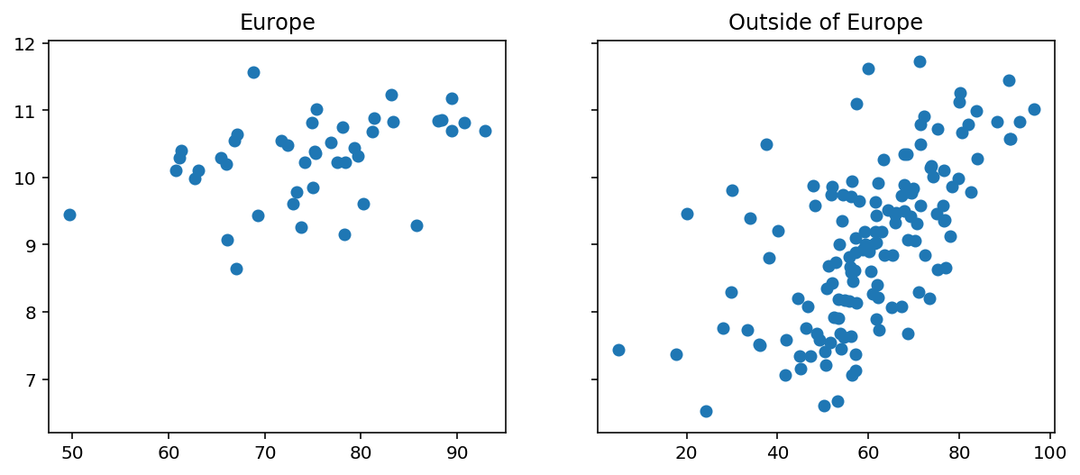
To supplement the model, we’ll also add an interaction term between business_freedom and is_europe and call it business_freedom_x_region. Here’s what the data looks like for countries inside and outside Europe.

Regression Model

Below is the regression model we have for our data that is based on observations $(X, y)$ and parameters $(\beta, \sigma)$.

Ordinary Linear Regression

Ordinary linear regression takes equation (1) and finds optimal values for $(\beta, \sigma)$ by minimizing the distance between the estimated value of $y$, and the observed value of $y$. Below is an implementation of the model in Sklearn and a plot of the regression lines for European and non-European nations.

features = ["business_freedom", "business_freedom_x_region", "is_europe"]
x = df[features]
y = df["log_gdppc"]

reg = LinearRegression()
_ = reg.fit(x, y)
coef = dict([i for i in zip(list(x.columns), reg.coef_)])
# code for posterior plots is in the notebook linked at the bottom of this post

# backout the slopes of the regression lines for nations in and out of Europe
print("Slope for European Nations: ",
      round(coef["business_freedom"] + coef["business_freedom_x_region"], 3))
print("Slope for non-European Nations: ", round(coef["business_freedom"], 3))

Slope for European Nations:  0.026
Slope for non-European Nations:  0.046

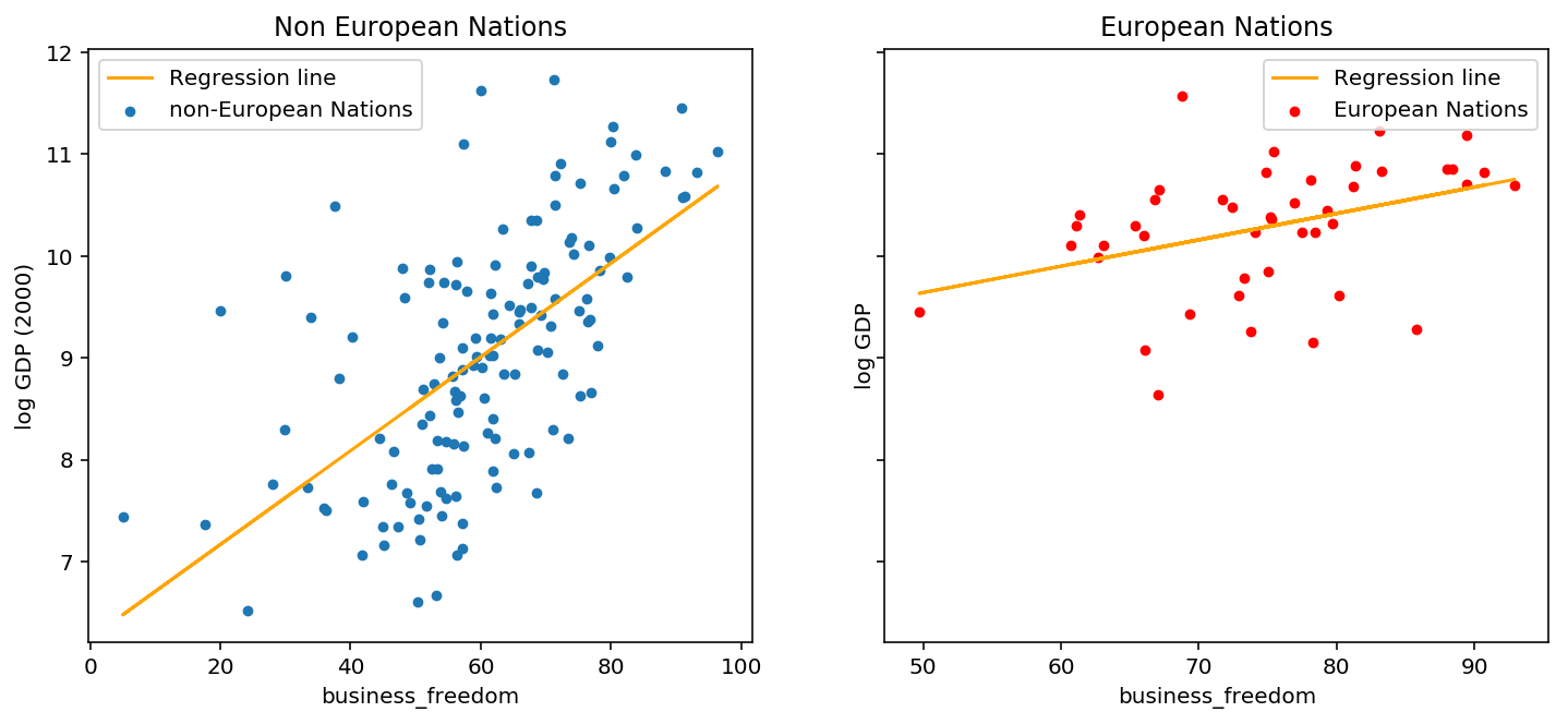
Although the slope for non-European countries is twice as large as European countries (0.046 VS 0.026), the absolute value of both numbers is small. Are these estimates really that different? Ideally we want a measure of confidence for each estimate, then we can be more sure that they are different. Keep this problem in mind for the next section and we’ll see how Bayesian regression solves it.

Bayesian Regression

Starting back from the regression model in (1), since $\epsilon$ is Normally distributed, $y$ is also Normally distributed in this model. So assuming that we have values for $(\beta, \sigma)$, we can write down a distribution for $y$. This is called the likelihood distribution.

Remember that we’re interested in estimating values for $\beta$ so that we can plug them back into our model and interpret the regression slopes. Before we get to estimating, the Bayesian framework allows us to add anything we know about our parameters to the model. In this case we don’t know anything about $\beta$ which is fine, but we know that $\sigma$ can’t be less than 0 because it is a standard deviation. This step is referred to as prior specification.

Since we don’t know anything about $\beta$, we’ll use an uninformative prior (think flat probability distribution) of $N(0, 5)$. For $\sigma$ we’ll use $U(0, 10)$, which ensures only positive values. The choice of $10$ as the upper bound here is somewhat arbitrary, the rational is that $\sigma$ probably won’t be very high based on the values of our response variable, $y$.

Now we want to get the distribution $p(\beta | y, \sigma)$, which is proportional to the likelihood (2) multiplied by the priors. This is called the posterior formulation. In real world applications, the posterior distribution is usually intractable (cannot be written down). Here’s where MCMC and variational inference come into play with Bayesian methods - they are used to draw samples from intractable posterior distributions, so that we can learn about our parameters. At this point you may be wondering why are we concerned with a distribution when $\beta$ is a number (vector of numbers). Well, the distribution gives us more information about $\beta$, then we can find point estimates by finding the mean, median, mode, etc.

To write the Bayesian model in Python, we’ll use Pyro. I skip over small details in the code, however Pyro has amazing examples in their docs if you want to learn more.

# specify the linear model
class BayesianRegression(PyroModule):
    def __init__(self, in_features, out_features):
        super().__init__()
        self.linear = PyroModule[nn.Linear](in_features, out_features)
        # PyroSample used to declare priors:
        self.linear.weight = PyroSample(dist.Normal(0., 5.).expand([out_features, in_features]).to_event(2))
        self.linear.bias = PyroSample(dist.Normal(0., 5.).expand([out_features]).to_event(1))

    def forward(self, x, y=None):
        sigma = pyro.sample("sigma", dist.Uniform(0., 10.))
        mean = self.linear(x).squeeze(-1)
        # sample from the posterior
        obs = pyro.sample("obs", dist.Normal(mean, sigma), obs=y)
        return mean

model = BayesianRegression(3, 1)
auto_guide = AutoDiagonalNormal(model)
svi = SVI(model = model, # bayesian regression class
          guide = auto_guide, # using auto guide
          optim = pyro.optim.Adam({"lr": 0.05}), # optimizer
          loss=Trace_ELBO()) # loss function

num_iterations = 2500
# param_store is where pyro stores param estimates
pyro.clear_param_store()
# inference loop
for j in range(num_iterations):
    # calculate the loss and take a gradient step
    loss = svi.step(x_data, y_data)
    if j % 250 == 0:
        print("[iteration %04d] loss: %.4f" % (j + 1, loss / len(data)))

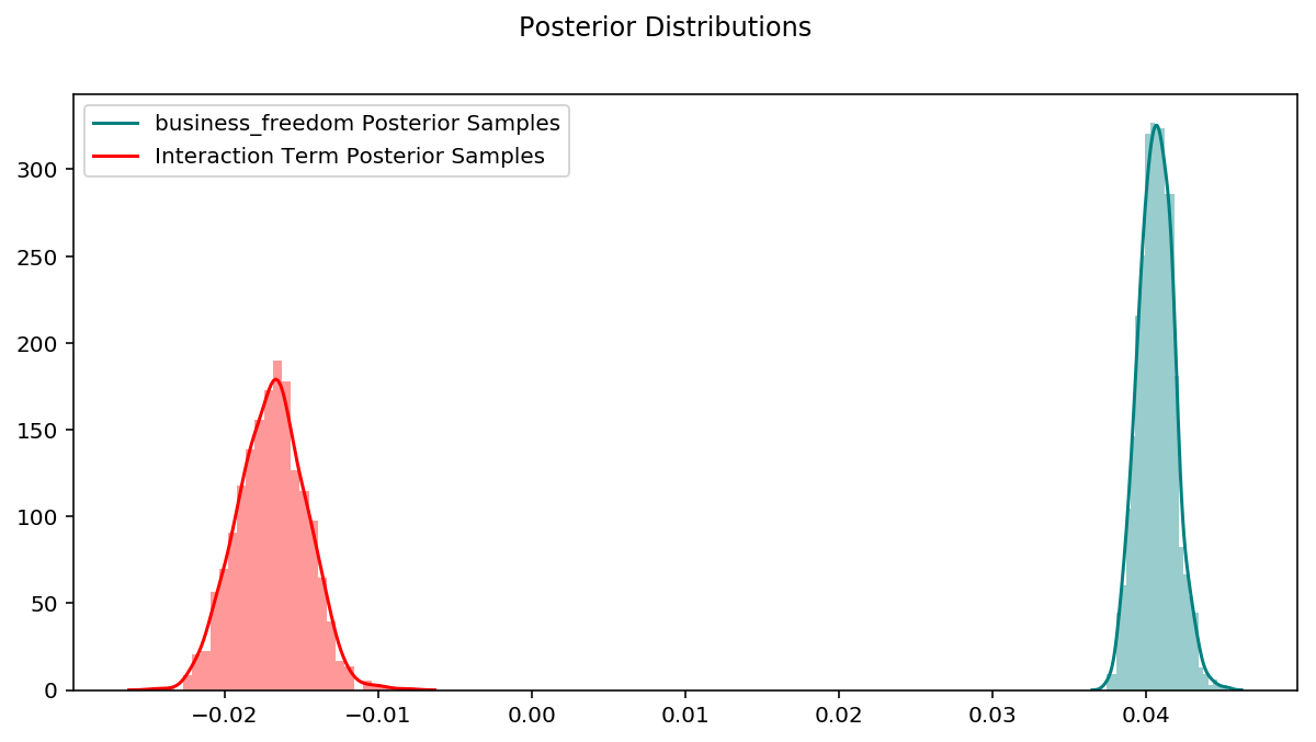
For posterior inference, we use stochastic variational inference, which is a method used to approximate probability distributions. The code above initializes the stochastic variational inference sampler and runs it for $2500$ iterations. Now the Predictive class can be used to generate posterior samples for each parameter. We’ll only plot the posterior distributions for business_freedom and business_freedom_x_region as these are the most important.

num_samples = 1000
predictive = Predictive(model = model,
                        guide = auto_guide,
                        num_samples = num_samples,
                        return_sites=("linear.weight", "linear.bias", "obs", "_RETURN"))
pred = predictive(x_data)
weight = pred["linear.weight"]
weight = weight.reshape(weight.shape[0], 3)
bias = pred["linear.bias"]
# code for posterior plots is in the notebook linked at the bottom of this post

Here is where the advantage of Bayesian linear regression starts to show. With Ordinary linear regression we end up with point estimates of parameters, but now we have an entire distribution for each parameter, and can use it to determine confidence levels. By combining appropriate posteriors and taking the mean, we can calculate a distribution for the slopes and compare them to the point estimates from ordinary linear regression.

slope_inside_europe = weight[:, 1] + weight[:, 2] # business_freedom + business_freedom_x_region
slope_outside_europe = weight[:, 1] # business_freedom

print("Slope for European nations: ", torch.mean(slope_inside_europe).numpy()) # business_freedom + interaction
print("Slope for non-European nations: ", torch.mean(slope_outside_europe).numpy()) # business_freedom

fig = plt.figure(figsize=(10, 5))
sns.distplot(slope_inside_europe, kde_kws = {"label": "European nations"})
sns.distplot(slope_outside_europe, kde_kws={"label": "Non-European nations"})
fig.suptitle("log(GDP Per Capita) vs Business Freedom");

Slope for European nations:  0.023792317
Slope for non-European nations:  0.040710554

These estimates are different to the ones from Ordinary linear regression. This is because of the priors we used in the Bayesian model. Neither method is necessarily “more correct”. Actually, if we were to specify all flat priors and sample from the true posterior distribution, the parameter estimates would be the same.

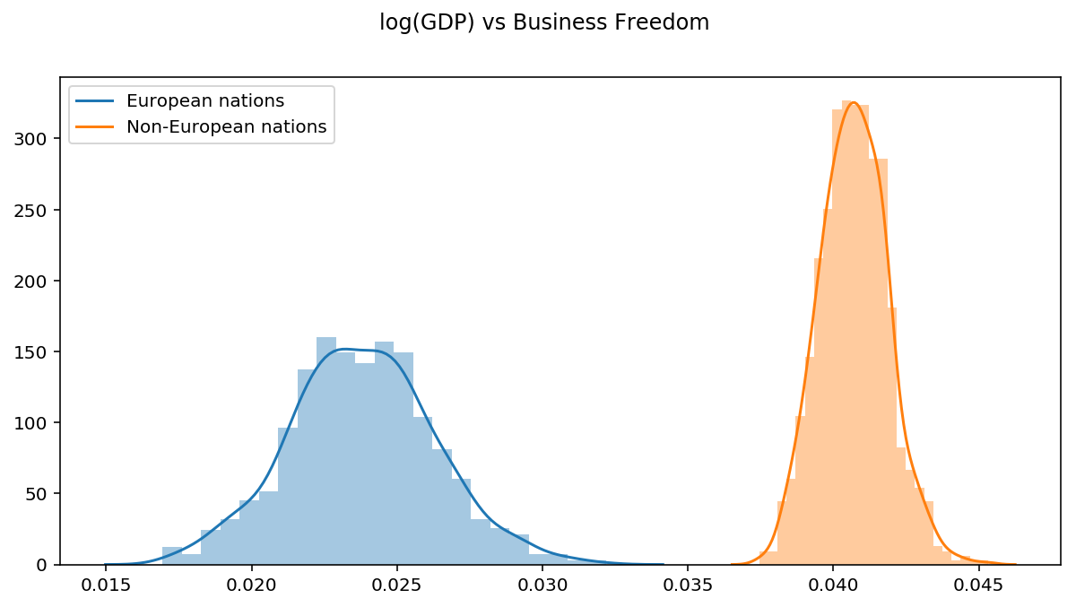
Although the absolute value of these slopes are small, we now have more confidence that the they are different becuase their distributions don’t overlap.

Returning to the questions we asked at the beginning of this post:

• Why should I even use this complicated black magic if other models are better? - Different tools for different jobs. Non-Bayesian models are not as expressive as their Bayesian counterparts. If all we care about is predictive power, then there’s little need for parameter confidence intervals and a non-Bayesian approach will suffice in most instances. However, when we want to do inference and compare effects (coefficients) with some level of confidence, Bayesian methods shine.
• Since when is there a Bayesian version of simple linear regression? - There’s a Bayesian version of most models. If we have a model for data that can be expressed as a probability distribution, then we can specify distributions for its parameters and come up with a Bayesian formulation.
• What in the world is MCMC and should I even care? - MCMC is a family of methods used to sample arbitrary probability distributions. In Bayesian problems, the posterior distribution is not usually well defined, so we use MCMC algorithms to sample them.

All the code for this blog post can be viewed here.