Problem
With the current global pandemic and its associated resources (data, analyses, etc.), I’ve been trying for some time to come up with an interesting COVID-19 problem to attack with statistics. After looking at the number of confirmed cases for some counties, it was clear that at some date, the number of new cases stopped being exponential and its distribution changed. However, this date was different for each country (obviously). This post introduces and discusses a Bayesian model for estimating the date that the distribution of new COVID-19 cases in a particular country changes.
An important reminder before we get into it is that all models are wrong, but some are useful. This model is useful for estimating the date of change, not for predicting what will happen with COVID-19. It should not be mistaken for an amazing epidemiology model that will tell us when the quarantine will end, but instead a way of describing what we have already observed with probability distributions.
All the code for this post can be found here.
Model
We want to describe $y$, log of the number of new COVID-19 cases in a particular country each day, as a function of $t$, the number of days since the virus started in that country. We’ll do this using a segmented regression model. The point at which we segment will be determined by a learned parameter, $\tau$. This is model is written below:
Likelihood:
\[\begin{equation*} \begin{split} y = wt + b + \epsilon \end{split} \text{, } \qquad \qquad \begin{split} \epsilon \sim N(0, \sigma^2) \\[10pt] p(y \mid w, b, \sigma) \sim N(wt, \sigma^2) \end{split} \\[15pt] \end{equation*}\] \[\begin{equation*} \begin{split} \text{Where: } \qquad \qquad \end{split} \begin{split} w &= \begin{cases} w_1 & \text{if } \tau \le t\\ w_2 & \text{if } \tau \gt t\\ \end{cases} \\ b &= \begin{cases} b_1 & \text{if } \tau \le t\\ b_2 & \text{if } \tau \gt t\\ \end{cases} \end{split} \\[10pt] \end{equation*}\]Priors:
\[\begin{equation*} w_1 \sim N(\mu_{w_1}, \sigma_{w_1}^2) \qquad \qquad w_2 \sim N(\mu_{w_2}, \sigma_{w_2}^2) \\[10pt] b_1 \sim N(\mu_{b_1}, \sigma_{b_1}^2) \qquad \qquad b_2 \sim N(\mu_{b_2}, \sigma_{b_2}^2) \\[10pt] \tau \sim Beta(\alpha, \beta) \qquad \qquad \sigma \sim U(0, 3) \end{equation*}\]
In other words, $y$ will be modeled as $w_1t + b_1$ for days up until day $\tau$. After that it will be modeled as $w_2t + b_2$.
The model was written in Pyro, a probabilistic programming language built on PyTorch. Chunks of the code are included in this post, but the majority of code is in this notebook.
Data
The data used was downloaded from Kaggle. Available to us is the number of daily confirmed cases in each country, and Figure 1 shows this data in Italy. It is clear that there are some inconsistencies in how the data is reported, for example, in Italy there are no new confirmed cases on March 12th, but nearly double the expected cases on March 13th. In cases like this, the data was split between the two days.
The virus also starts at different times in different countries. Because we have a regression model, it is inappropriate to include data prior to the virus being in a particular country. This date is chosen by hand for each country based on the progression of new cases and is never the date the first patient is recorded. The “start” date is better interpreted as the date the virus started to consistently grow, as opposed to the date the patient 0 was recorded.
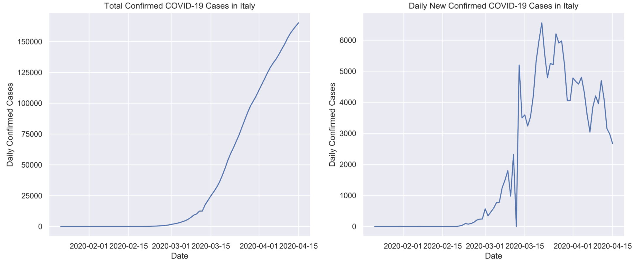
Total confirmed COVID-19 cases in Italy on the left and daily cases on the right, from January 1st to March 15th 2020
Prior Specification
Virus growth is sensitive to population dynamics of individual countries and we are limited in the amount of data available, so it is important to supplement the model with appropriate priors.
Starting with $w_1$ and $w_2$, these parameters can be loosely interpreted as the growth rate of the virus before and after the date change. We know that the growth will be positive in the beginning and is not likely to be larger than $1$. With these assumptions, $w_1 \sim N(0.5, 0.25)$ is a suitable prior. We’ll use similar logic for $p(w_2)$, but will have to keep in mind flexibility. Without a flexible enough prior here, the model won’t do well in cases where there is no real change point in the data. In these cases, $w_2 \approx w_1$, and we’ll see and example of this in the Results section. For now, we want $p(w_2)$ to be symmetric about $0$, with the majority of values lying between $(-0.5, 0.5)$. We’ll use $w_2 \sim N(0, 0.25)$.
Next are the bias terms, $b_1$ and $b_2$. Priors for these parameters are especially sensitive to country characteristics. Countries that are more exposed to COVID-19 (for whatever reason), will have more confirmed cases at its peak than countries that are less exposed. This will directly affect the posterior distribution for $b_2$ (which is the bias term for the second regression). In order to automatically adapt this parameter to different countries, we use the mean of the first and forth quartiles of $y$ as $\mu_{b_1}$ and $\mu_{b_2}$ respectively. The standard deviation for $b_1$ is taken as $1$, which makes $p(b_1)$ a relatively flat prior. The standard deviation of $p(b_2)$ is taken as $\frac{\mu_{b_2}}{4}$ so that the prior scales with larger values of $\mu_{b_2}$.
\[b_1 \sim N(\mu_{q_1}, 1) \qquad \qquad b_2 \sim N(\mu_{q_4}, \frac{\mu_{q_4}}{4}) \notag\]As for $\tau$, since at this time we don’t have access to all the data (the virus is ongoing), we’re unable to have a completely flat prior and have the model estimate it. Instead, the assumption is made that the change is more likely to occur in the second half of the date range at hand, so we use $\tau \sim Beta(4, 3)$.
class COVID_change(PyroModule):
    def __init__(self, in_features, out_features, b1_mu, b2_mu):
        super().__init__()
        self.linear1 = PyroModule[nn.Linear](in_features, out_features, bias = False)
        self.linear1.weight = PyroSample(dist.Normal(0.5, 0.25).expand([1, 1]).to_event(1))
        self.linear1.bias = PyroSample(dist.Normal(b1_mu, 1.))

        self.linear2 = PyroModule[nn.Linear](in_features, out_features, bias = False)
        self.linear2.weight = PyroSample(dist.Normal(0., 0.25).expand([1, 1])) #.to_event(1))
        self.linear2.bias = PyroSample(dist.Normal(b2_mu, b2_mu/4))

    def forward(self, x, y=None):
        tau = pyro.sample("tau", dist.Beta(4, 3))
        sigma = pyro.sample("sigma", dist.Uniform(0., 3.))
        # fit lm's to data based on tau
        sep = int(np.ceil(tau.detach().numpy() * len(x)))
        mean1 = self.linear1(x[:sep]).squeeze(-1)
        mean2 = self.linear2(x[sep:]).squeeze(-1)
        mean = torch.cat((mean1, mean2))
        obs = pyro.sample("obs", dist.Normal(mean, sigma), obs=y)
        return mean
Hamiltonian Monte Carlo is used for posterior sampling. The code for this is shown below.
model = COVID_change(1, 1,
                     b1_mu = bias_1_mean,
                     b2_mu = bias_2_mean)

num_samples = 800
# mcmc
nuts_kernel = NUTS(model)
mcmc = MCMC(nuts_kernel,
            num_samples=num_samples,
            warmup_steps = 100,
            num_chains = 4)
mcmc.run(x_data, y_data)
samples = mcmc.get_samples()
Results
Since I live in Canada and have exposure to the dates precautions started, modeling will start here. We’ll use February 27th as the date the virus “started”.
Priors:
\[w_1, w_2 \sim N(0, 0.5) \qquad b_1 \sim N(1.1, 1) \qquad b_2 \sim N(7.2, 1) \notag\]
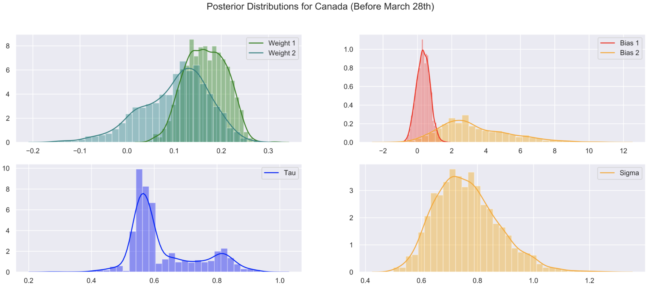
Posterior Distributions
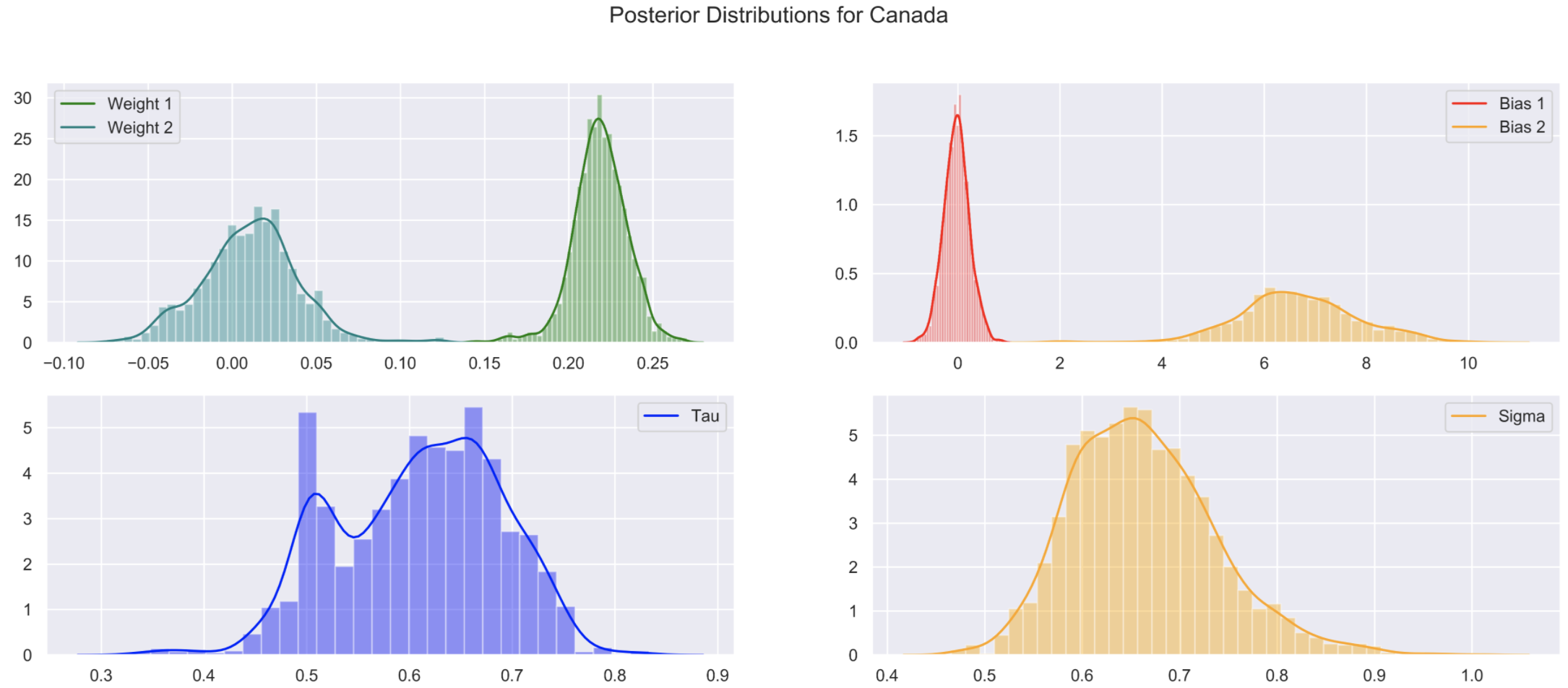
Posterior distributions for each parameter in our model using Canada's COVID-19 data. Notice that the posteriors for $w_1$ and $w_2$ don't overlap
Starting with the posteriors for $w_1$ and $w_2$, if there was no change in the data we would expect to see these two distributions close to each other as they govern the growth rate of the virus. It is a good sign that these distributions, along with the posteriors for $b_1$ and $b_2$, don’t overlap. This is evidence that the change point estimated by our model is true.
This change point was estimated as: 2020-03-28
As a side note, with no science attached, my company issued a mandatory work from home policy on March 16th. Around this date is when most companies in Toronto would have issues mandatory work from home policies where applicable. Assuming the reported incubation period of the virus is up to 14 days, this estimated date change makes sense as it is 12 days after widespread social distancing measures began!
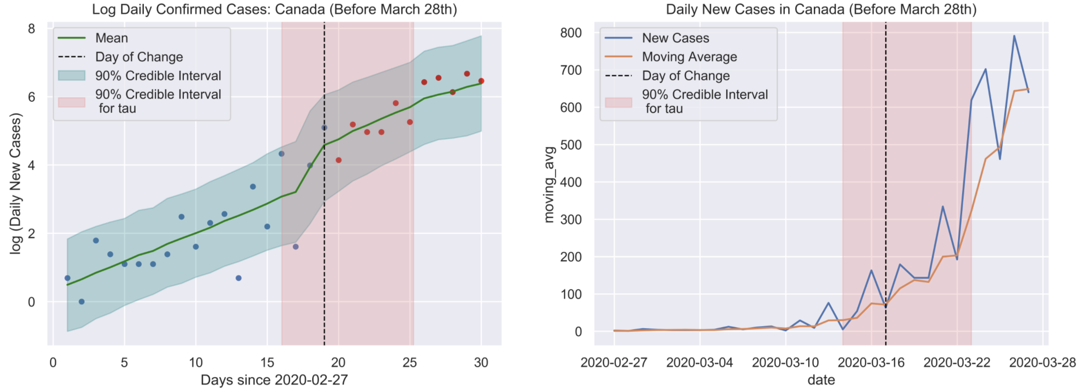
The model fit along with 95% credible interval bands can be seen in the plot below. On the left is log of the number of daily cases, which is what we used to fit the model, and on the right is the true number of daily cases. It is very difficult to visually determine a change point by simply looking at the number of daily cases, and even more difficult by looking at the total number of confirmed cases.
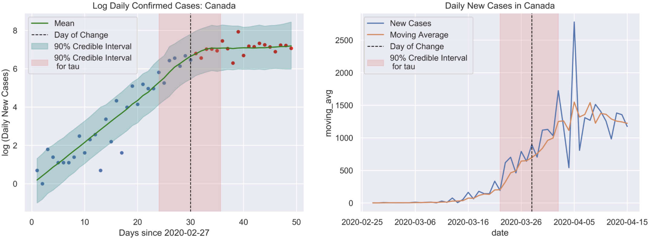
Left: log(daily confirmed cases) with the estimated date that the curve started to flatten (March 28th) and the 90% credible interval. Right: Raw data for the daily cases each day, along with a 90% credible interval for the day the curve started to flatten
Assessing Convergence
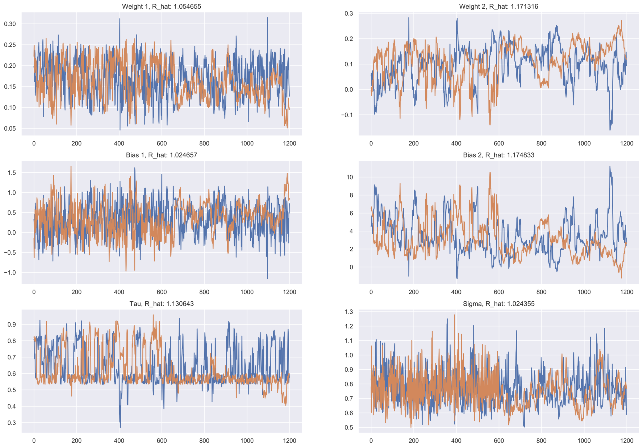
When running these experiments, the most important step is to diagnose the MCMCfor convergence. I adopt 3 ways of assessing convergence for this model by observing mixing and stationarity of the chains and $\hat{R}$. $\hat{R}$ is the factor by which each posterior distribution will reduce by as the number of samples tends to infinity. A perfect $\hat{R}$ value is 1, and values less than $1.1$ are indicative of convergence. We observe mixing and stationarity of the Markov chains in order to know if the HMC is producing appropriate posterior samples.
Below are trace plots for each parameter. Each chain is stationary and mixes well. Additionally, all $\hat{R}$ values are less than $1.1$.
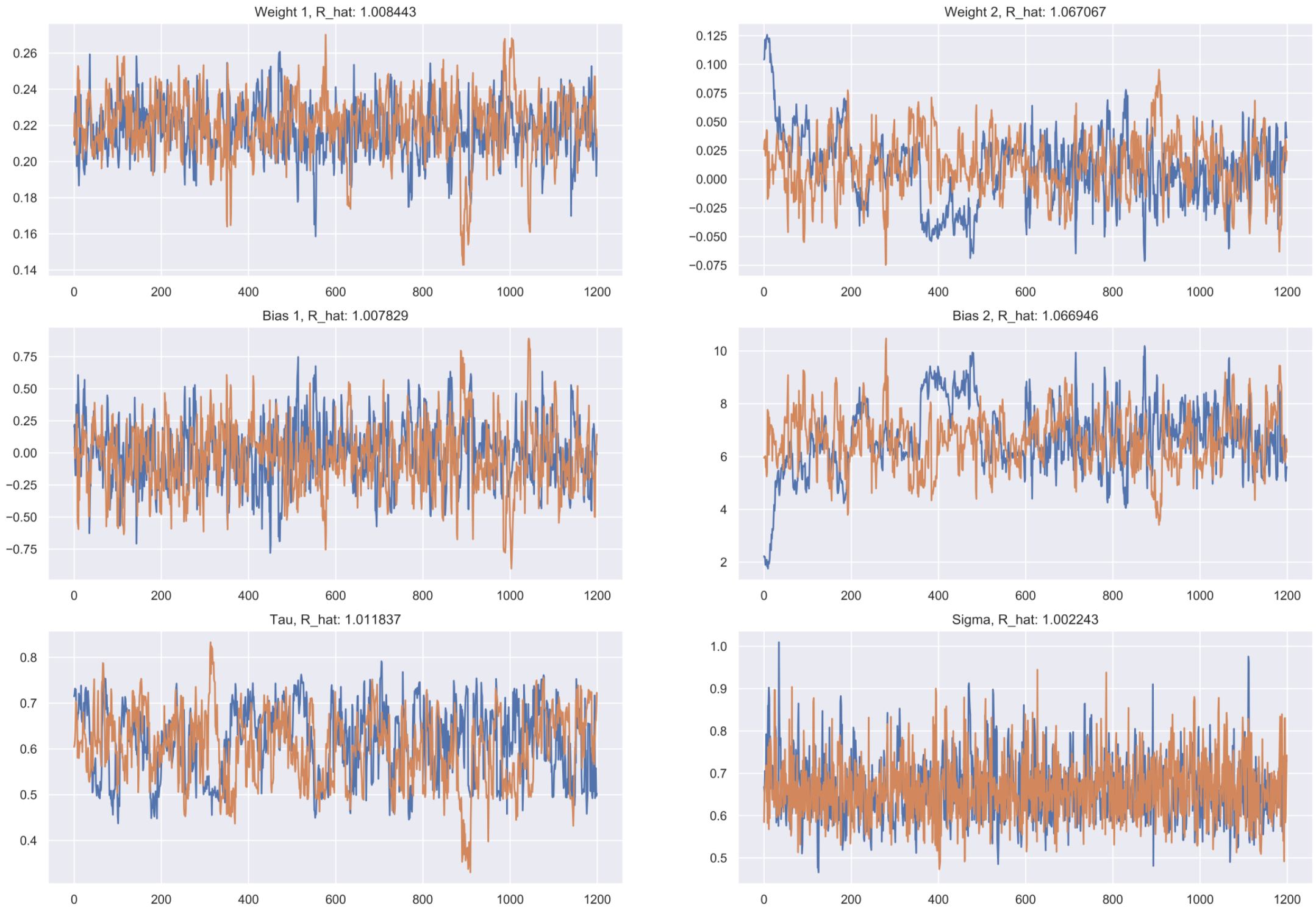
Trace plots and $\hat{R}$ values for all posterior samples, plotten for MCMC diagnostics.
After convergence, the last thing to check before moving on to other examples is how appropriate the model is for the data. Is it consistent with the assumptions made earlier? To test this we’ll use a residual plot and a QQ-plot, as shown below. I’ve outlined the estimated change point in order to compare residuals before and after the change to test for homoscedasticity. The residuals follow a Normal distribution with zero mean, and no have dependence with time, before and after the date of change.
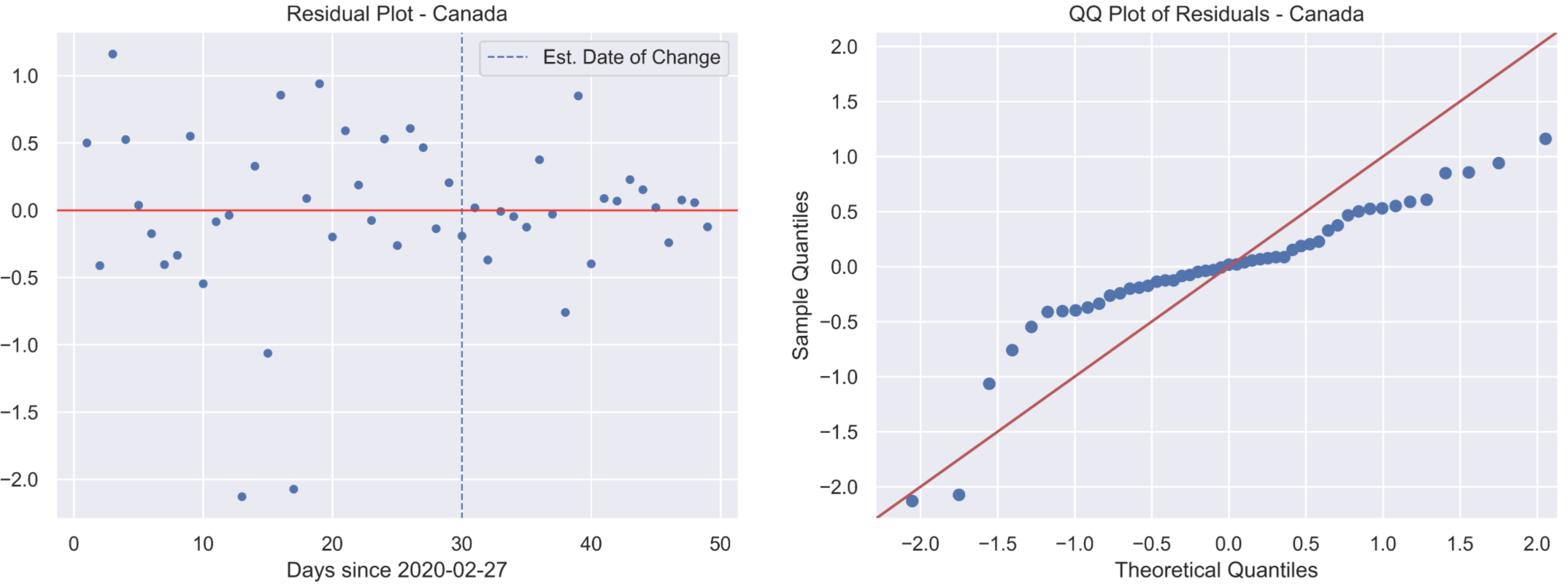
Residual and QQ-plots validating our error assumption.
What About no Change?
To test the model’s robustness to a country that has not began to flatten the curve, we’ll look at data from Canada up until March 28th. This is the day that the model estimated curve flattening began in Canada. Just because there isn’t a true change date doesn’t mean the model will output “No change”. We’ll have to use the posterior distributions to reason that the change date provided by the model is inappropriate, and consequentially there is no change in the data.
Prior
\[w_1, w_2 \sim N(0, 0.5) \qquad b_1 \sim N(0.9, 1) \qquad b_2 \sim N(6.4, 1.6) \notag\]
Posterior Distributions
Posterior plots for parameters after selecting a date range where the COVID-19 curve has not began to flatten. Notice the distributions for $w_1$ and $w_2$ overlap
The posteriors for $w_1$ and $w_2$ have significant overlap, indicating that the growth rate of the virus hasn’t changed significantly. Posteriors for $b_1$ and $b_2$ are also overlapping. These show that the model is struggling to estimate a reasonable $\tau$, which is good validation for us that the priors aren’t too strong.
Although we have already concluded that there is no change date for this data, we’ll still plot the model out of curiosity.
Similar to the previous example, the MCMC has converged. The trace plots below show sufficient mixing and stationarity of the chains, and most $\hat{R}$ values less than $1.1$.
Next Steps and Open Questions
This model is able to describe the data well enough to produce a reliable estimate of the day flattening the curve started. An interesting byproduct of this is the coefficient term for the 2nd regression line, $w_2$. By calculating $w_2$ and $b_2$ for different countries, we can compare how effective their social distancing measures were. The logical next modelling step would be to fit a hierarchical model in order to use partial pooling of data between countries.
Thank you for reading, and definitely reach out to me by e-mail or other means if you have suggestions or recommendations, or even just to chat!