This post motivates the Beta and Dirichlet distributions using a simple example. It also relates the Beta and Dirichlet distributions to the Binomial and Multinomial. It’s written without any equations for readability.
Throughout the post, we’ll use probability distributions to model people’s favourite color. The favourite color experiments start off very simple, then get more interesting as we introduce more flexible probability distributions. Then we briefly touch on how the Dirichlet distribution works.
Binomial Distribution
The Binomial distribution describes the number of successes in a binary task. It is parametized by the probability of success, $p$, and the number of times the task was completed, $n$.
Example: Simple Favourite Colour
Suppose we have an experiment where we ask $n$ random people if their favourite color is blue. The number of people whose favourite colour is blue, follows a Binomial distribution. The parameter $p$ being the probability of someone’s favourite color being blue. Taking $p=0.5$ and $n=1000$, we can sample from this Binomial and each sample is a potential number of people whose favourite color is blue.
from scipy.stats import binom

binom_rvs = binom.rvs(n= 1000, p = 0.5, size=5000)

fig, ax = plt.subplots(nrows=1, ncols=1, figsize=(6, 4), sharex = True)
sns.distplot(binom_rvs, kde = False, bins = 20)
plt.title("Samples from a Binomial(n=1000, p=0.5)")
plt.xlabel("Number of Successes")
plt.ylabel("Density")
plt.yticks([]);
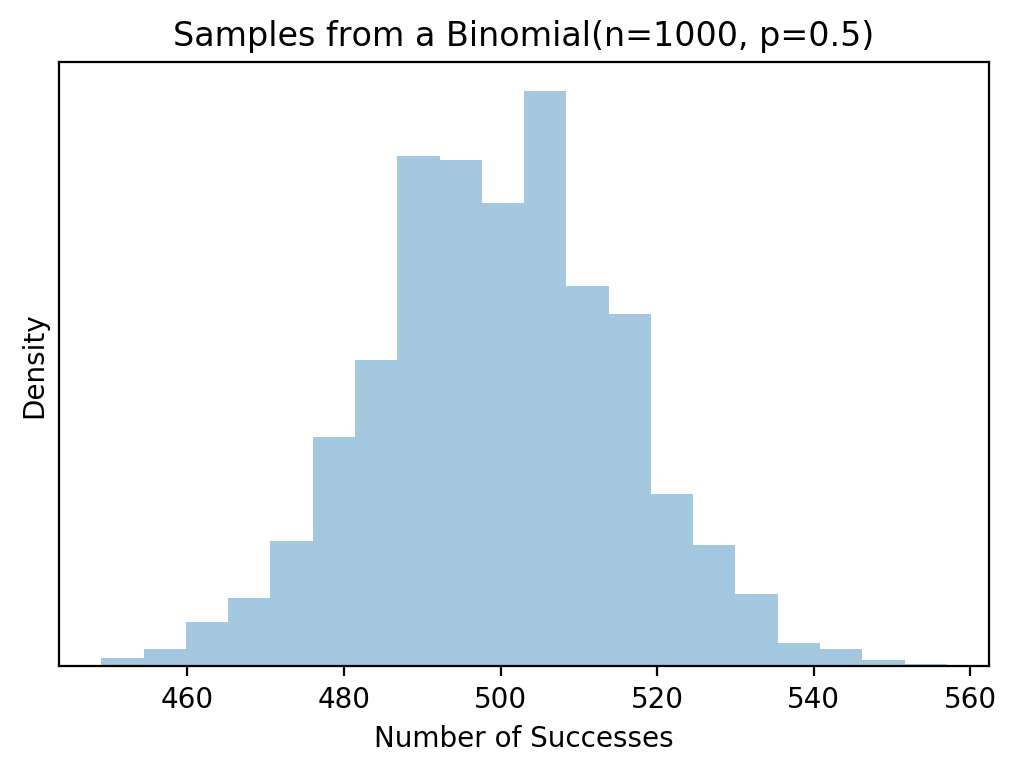
Histogram of samples from a Binomial(n=1000, p=0.5) distribution. The mean of this distribution is 500, so we expect histogram to be centered around 500, which it is. This of course corresponds to an average of 500 successes over 1000 tries, with a probability of success of 0.5
Beta Distribution
In a Bayesian setting, we’ll want to use the Binomial distribution as the likelihood for the favourite color problem mentioned above. This would mean placing a prior on $p$, which is a probability and needs to be between $[0, 1]$. It’s possible to use any probability density whose domain is $[0,1]$, however we prefer a distribution that would leave us with an analytic posterior. For a Binomial likelihood this is the Beta distribution, meaning Beta is a conjugate prior for the Binomial.
Samples from the Beta distribution can be thought of as potential probabilities of success, $p$, for the Binomial. The Beta distribution itself is parameterized by $(\alpha, \beta)$ which determine its location and scale. Below are plots of samples from the Beta distribution with different parameters, notice that all the samples are between $(0, 1)$.
from scipy.stats import beta

n = int(5e5) # number of samples
fig, ax = plt.subplots(nrows=2, ncols=2, figsize=(8, 5), sharex = True)

sns.distplot(beta.rvs(2, 2, size = n),
             hist = False,
#             color="r",
             kde_kws={"shade": True},
             ax = ax[0, 0]).set_title("Samples from Beta(2,2)")

sns.distplot(beta.rvs(4, 4, size = n),
             hist = False,
             kde_kws={"shade": True},
             ax = ax[0, 1]).set_title("Samples from Beta(4, 4)")

sns.distplot(beta.rvs(2, 4, size = n),
             hist = False,
             kde_kws={"shade": True},
             ax = ax[1, 0]).set_title("Samples from Beta(2, 4)")

sns.distplot(beta.rvs(4, 2, size = n),
             hist = False,
             kde_kws={"shade": True},
             ax = ax[1, 1]).set_title("Samples from Beta(4, 2)");
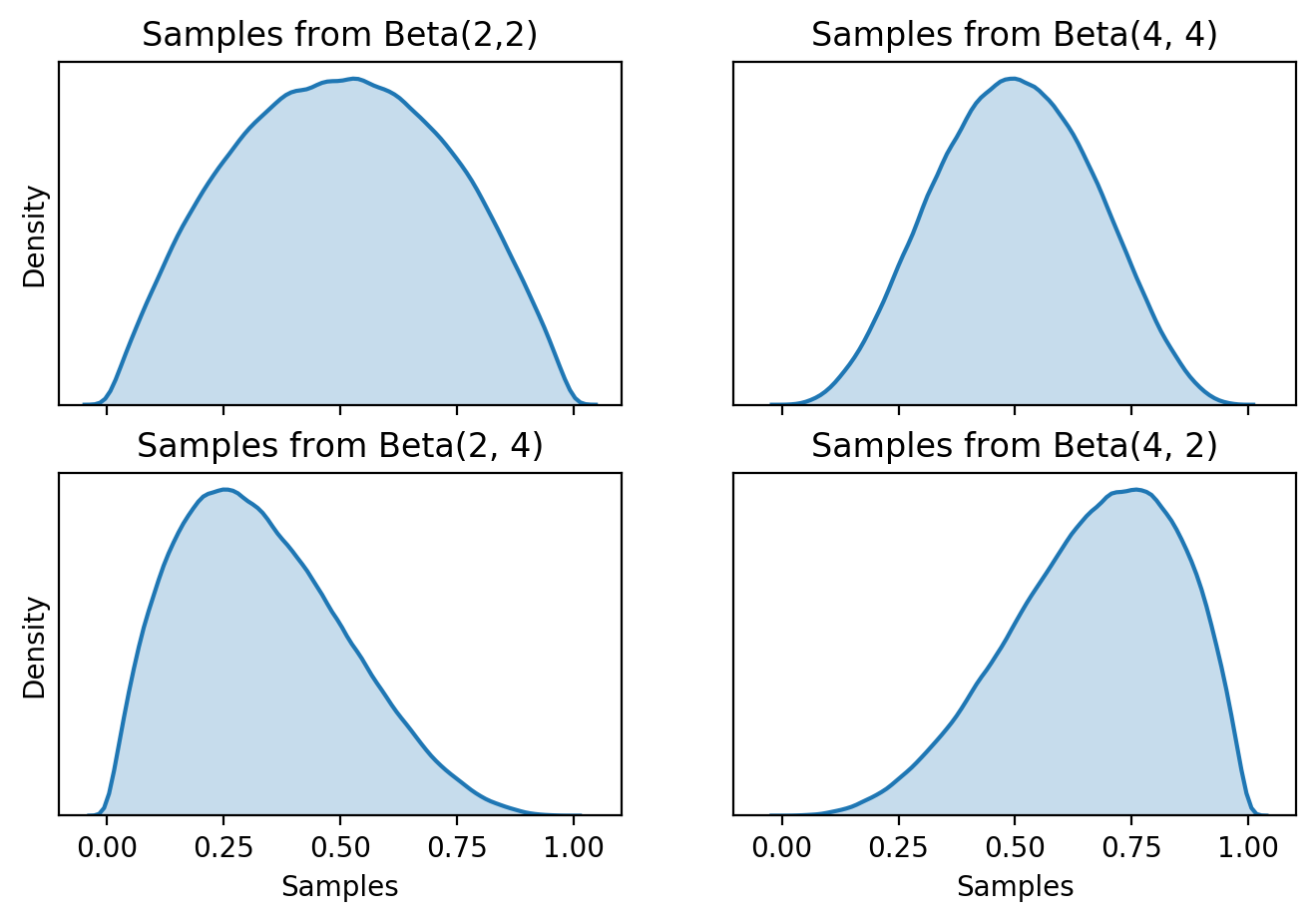
Plots for 4 different specifications of the Beta distribution. Notice on the x-axis that the support is between [0, 1]
Multinomial Distribution
A limitation of the Binomial distribution is we only have 2 potential outcomes. The Multinormial distribution is a generalization of this, so we can have $k$ possible outcomes. It is parameterized by the number of trials, $n$ and the probability of success for each outcome $p_i$. Each sample from a Multinomial is a vector of length $k$, where each index corresponds to the number of successes for that outcome.
Example: Favourite Colour
We used the Binomial distribution to find out if people’s favourite colour is blue, but this didn’t give us much information on what other colours people liked. Now we want more information. We’re interested in the distribution of people whose favourite colours are either: blue, green, red or yellow. If we ask $n$ people to choose their favourite color from one of these, the number of successes for each colour will follow a Multinomial distribution. Each parameter, $p_{blue}, p_{green}, p_{red}, p_{yellow}$ is the probability of that colour being a random person’s favourite. Sampling from this Multinomial will return a vector of length $4$ corresponding to the number of successes for that color. For each sample, the total number of successes sums to $n$.
from scipy.stats import multinomial

_p = [0.1, 0.15, 0.25, 0.5]
multinom_rvs = multinomial.rvs(n=1000, p=_p, size = 10000)

fig, ax = plt.subplots(nrows=1, ncols=1, figsize=(7, 4), sharex = True)
sns.distplot(multinom_rvs[:, 0],
             hist = False,
             kde_kws={"label": "Class 1", "shade": True})

sns.distplot(multinom_rvs[:, 1],
             hist = False,
             kde_kws={"label": "Class 2", "shade": True})

sns.distplot(multinom_rvs[:, 2],
             hist = False,
             kde_kws={"label": "Class 3", "shade": True})

sns.distplot(multinom_rvs[:, 3],
             hist = False,
             kde_kws={"label": "Class 4", "shade": True}).set_title("Multinomial Samples for class 4, p=[0.1, 0.15, 0.25, 0.5]");
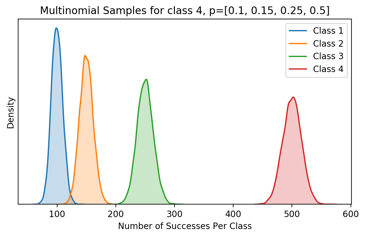
Histogram of samples from a Multinomial distribution with 4 classes, and probabilities: [0.1, 0.15, 0.25, 0.5].
Dirichlet Distribution
Similarly with the Beta and Binomial combo, we need a prior for each $p_i$ in the Multinomial likelihood. Unlike the Binomial, where we could potentially use any distribution with $(0, 1)$ domain as a prior for $p$, the Multinomial has an added restriction, as the vector of probabilities needs to sum to 1. Placing an arbitrary prior on each $p_i$ won’t ensure that $\sum p_i = 1$. This is what the Dirichlet distribution offers. It acts as a prior over the entire vector of probabilities, $p = [p_1, p_2, …, p_k]$. It is a generalization of the Beta distribution, and is also a conjugate prior for the Multinomial, which is an added benefit.
A vector of length $k$ parameterizes the Dirichlet distribution, and the parameters are similar to $(\alpha, \beta)$ for the Beta distribution. Below are samples from 2 Dirichlet distributions with different parameters.
from scipy.stats import dirichlet

dirich_samples = pd.DataFrame(dirichlet.rvs(alpha = [1, 5, 15], size = 10000))

fig, ax = plt.subplots(nrows=2, ncols=1, figsize=(8, 5), sharex = True)

sns.distplot(dirich_samples[0],
             kde_kws = {"label": "Alpha = 1", "shade": True},
             color = "teal",
             hist = False,
             ax = ax[0],
             kde = True)
sns.distplot(dirich_samples[1],
             kde_kws = {"label": "Alpha = 5", "shade": True},
             color = "blue",
             hist = False,
             ax = ax[0],
             kde = True)
sns.distplot(dirich_samples[2],
             kde_kws = {"label": "Alpha = 15", "shade": True},
             color = "red",
             hist = False,
             ax = ax[0],
             kde = True)
ax[0].set_title("Samples from Dir([1, 5, 15])")
ax[0].set_yticks([])
ax[0].set_xlabel("")
ax[0].set_ylabel("Density")

dirich_samples = pd.DataFrame(dirichlet.rvs(alpha = [10, 0.5, 7], size = 10000))
sns.distplot(dirich_samples[0],
             kde_kws = {"label": "Alpha = 10", "shade": True},
             color = "teal",
             hist = False,
             ax = ax[1],
             kde = True)
sns.distplot(dirich_samples[1],
             kde_kws = {"label": "Alpha = 0.5", "shade": True},
             color = "blue",
             hist = False,
             ax = ax[1],
             kde = True)
sns.distplot(dirich_samples[2],
             kde_kws = {"label": "Alpha = 7", "shade": True},
             color = "red",
             hist = False,
             ax = ax[1],
             kde = True)
ax[1].set_title("Samples from Dir([10, 0.5, 7])")
ax[1].set_xlabel("Samples")
ax[1].set_yticks([])
ax[1].set_ylabel("Density");
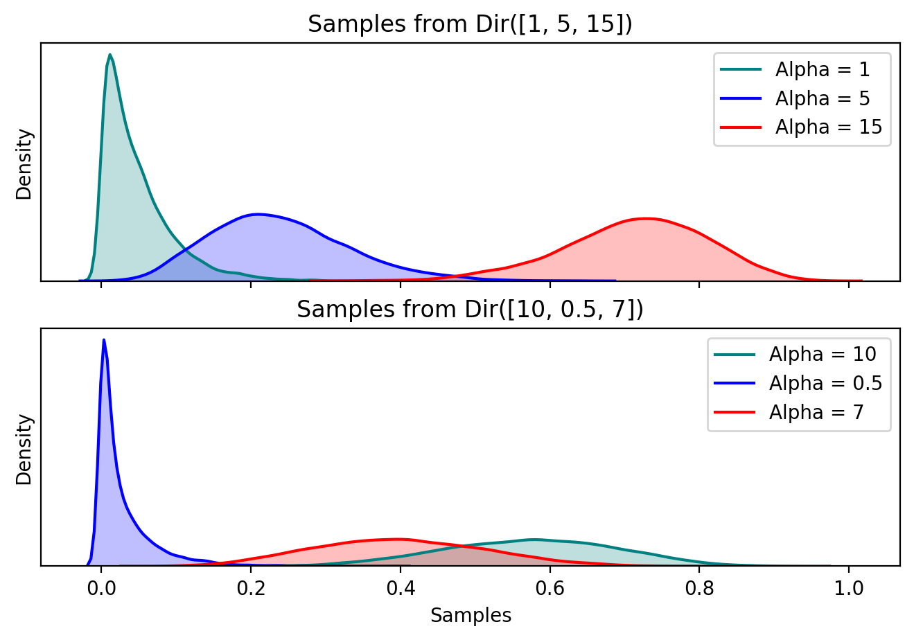
Probability distributions for 2 different Dirichlet distributions, one above and another below. Notice that the support of the entire distribution is [0, 1], similar to the Beta. It cannot be seen on the graph, but each sample in the Dirichlet sums to 1.
How do we always sum to 1?
Let’s take a Dirichlet distribution with 5 components, meaning that samples from this distribution will be a vector of length 5, whose sum is 1:
\[X \sim Dir([\alpha_1, \alpha_2, \alpha_3, \alpha_4, \alpha_5]) \notag\]Two samples from $X$:
\[x_1 = [0.3, 0.15, 0.05, 0.25, 0.25] \notag\] \[x_2 = [0.13, 0.17, 0.05, 0.2, 0.45] \notag\]Two things are consistent: $\sum_{i=1}^{5} x_i = 1$ and len(x) = $5$. So we can imagine that each sample from a Dirichlet distribution is a literal stick of length 1, that is broken into $5$ sections. Each section (or class) has a length, for example section 2 in $x_1$ has length $0.15$. Each sample can have different lengths for each section. The Dirichlet distribution does is proposes different ways of breaking this stick into 5 pieces. Of course, there is a specific way of breaking the stick to generate samples from the Distribution, which is very aptly named the stick breaking construction.
The next logical step from here is to ask the question: why 5 pieces? What if we don’t know how many pieces we want? So really we want a distribution to propose breaking this stick in any way possible, 3 pieces, 100 pieces, 1e10 places. This can be done with a Dirichlet process.
Another View: Distribution over Distributions
Suppose we have an arbitrary experiment with $k$ outcomes, that each happen with probability $p_i$. Every time we repeat this experiment, we get a probability distribution, $p$. Since we have a finite number of outcomes, we can imagine that each $p$ came from some Dirichlet distribution. In this sense, the Dirichlet distribution is a distribution over probability distributions.
Good resources for further reading: