Gaussian Processes and Regression

I’ve found many articles about Gaussian processes that start their explanation by describing stochastic processes, then go on to say that a GP is a distribution over functions, or an infinite dimensional distribution, etc. etc. I find these harsh for an introduction, so in this post I try to explain GPs in a more approachable manner. Then I talk about Gaussian process regression and its relationship with Bayesian linear regression, with a simple example using GPyTorch.

How to start thinking about a Gaussian Process?

We can start by building multivariate Gaussians from univariate Gaussians. With a single random variable, $X_1 \sim N(\mu_1, \sigma_1^2)$, we can append $X_2 \sim N(\mu_2, \sigma_2^2)$ to get the vector $(X_1, X_2)$. If $X_1$ and $X_2$ have covariance $\sigma_{12}$, this vector will have distribution:

If we continue appending more Normally distributed random variables, $X_3, X_4, …$ constructing larger multivariate Gaussians is easy, once we have their mean and covariance. Then, this multivariate Gaussian will be fully specified by the mean vector and covariance matrix. To generalize this concept of continuously incorporating Normally distributed RV’s into the same distribution, we need a function to describe the mean and another to describe the covariance.

This is what the Gaussian process provides. It is specified by a mean function, $\mu(x)$ and a covariance function (called the kernel function), $k(x, x’)$, that returns the covariance between two points, $x$ and $x’$. Now we are not limited to $n$ variables for a $n$-variate Gaussians, but can model any amount (possibly infinite) with the GP. We write:

The kernel function, $k(x, x’)$ is simply a measure of how similar $x$ and $x’$ are, and an exmaple of one is the squared exponential kernel:

This is a loose intro to GP’s to convey the interpretation of “infinite dimensional” and “distribution over functions”. The book Gaussian Processes for Machine Learning goes into detail.

Samples from a Gaussian Process Prior

Since the Gaussian process is essentially a generalization of the multivariate Gaussian, simulating from a GP is as simple as simulating from a multivariate Gaussian. The steps are below:

• Start with a vector, $x_1, x_2, …, x_n$ that we will build the GP from. This can be done in Python with np.linspace.
• Choose a kernel, $k$, and use it to calculate the covariance matrix for each combination of $(x_i, x_j)$. We should end up with a matrix of dimension $(n, n)$. This is the covariance matrix for the multivariate Gaussian we are sampling from. We’ll use a zero-vector for its mean
• The resulting sample paths from this multivariate Gaussian are realizations of the Gaussian process, $GP(0, k)$. We can plot these values and a 95% confidence interval by taking the mean $\pm$ 1.96.

Code to do this is below:

kernel = 1.0 * RBF(1.0)

n = 100 
n_func = 7 # number of functions to sample from the GP 
L = -5; U = 5

# start with X = (x_1, x_2, ..., x_n)
X = np.linspace(L, U, n).reshape(-1, 1)

#  use kernel to calculate the covariance matrix
K = kernel(X)

# parametize a multivariate Gaussian with zero mean and K as the covariance matrix
ys = multivariate_normal.rvs(mean = np.zeros(n), 
                             cov = K, 
                             size = n_func)

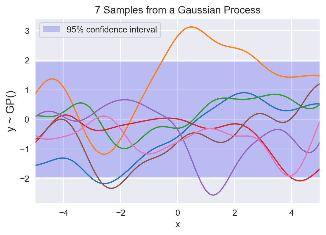
7 samples from a Gaussian process prior, along with a 95% confidence interval. Each curve is the result of sampling from a multivariate Gaussian with $n=100$ variables. If we reduce $n$, the samples will look less and less smooth, until $n=2$, where the sample will just be a line.

Gaussian Process + Regression

Nothing so far is groundbreaking, or particularly useful. All we have done is explained a way of generalizing the multivariate Normal, but haven’t talked about how it can be used in real life. However, you could imagine that starting with a prior over functions, we can form a posterior, $p(f \mid X, y)$ by conditioning on our data. Intiutively, doing this excludes all functions that don’t “pass through” our data, $(X, y)$.

I’ll approach Gaussian process regression from a slightly different perspective in this section, building up from Bayesian linear regression. This is a cool approach I found in David MacKay’s book, that I haven’t seem much elsewhere.

To set the stage, we are interested in modelling a function, $f$, for which we have data, $(X, y)$. We start with a feature map for the input, $R = \phi(X)$, so that $R$ an $N \times D$ matrix. Then $y = Rw$ and we can assign priors, $p(w)$, to build a posterior distribution for the weights, $p(w \mid y, X)$. This posterior is used to make future predictions and recreate $f = y + \epsilon$.

However, in some cases we’re only interested in making predictions, and in a Bayesian setting this boils down to 2 distributions: (1) the posterior predictive distribution in order to actually make a prediction and (2) the marginal likelihood for model comparison.

Expanding the formulations from Bayesian linear regression:

And since $y$ is a linear function of $w$ (which is a Normally distributed random variable), its prior is:

Accounting for noise in our observations, $\sigma^2_{err}$ the prior on our function, $f$, is:

This is how the Gaussian process is a prior over functions. The kernel described in that section is exacly $RR^T = \phi(X)\phi(X)^T$ in this section. Now we can start to create the posterior predictive distribution and marginal likelihood.

Before we get to the practical stuff, a note about kernels. There are many ways to get confused when first learning about kernels. What helped me is first understanding that a kernel is just a function that accepts 2 inputs and returns how “close” the inputs are to each other. From there, you can go in any direction exploring them, some good articles are: here, here and here.

Simulation Problem

In the first couple sentences of the last section I mentioned that we can condition the GP prior on the observed data to get a posterior distribution. All the observed data will then pass through this posterior distribution over functions. This section will use GP’s to extrapolate a simulated function. We don’t account for noisy observations, which is of course a terrible assumption in the real world.

I’ll use GPyTorch for inference. This is sort of like using a Ferrari to get groceries but GPyTorch looks promising, especially with Pytorch integration. Both PyMC3 and sklearn have easy-to-use implementations.

Here’s the function we want to approximate. The points in red are the training data, and we will try to approximate the blue section using a GP.

g = np.vectorize(lambda y: math.exp(-0.4 * y)*math.sin(4*y) + math.log(abs(y) + 1) + 1)
train_x = np.linspace(0, 4, 750)
test_x = np.linspace(4.01, 6, 100)
train_x = torch.tensor(train_x)
test_x = torch.tensor(test_x)

train_y = g(train_x) 
test_y = g(test_x) 
train_y=torch.tensor(train_y)
test_y=torch.tensor(test_y)

plt.figure(figsize=(6, 4), dpi=100)
sns.lineplot(train_x, train_y, color = 'red', label = "Train set")
sns.lineplot(test_x, test_y, color = 'blue', label = "Test set")
plt.title("Observed and test data")
plt.legend()
plt.show();

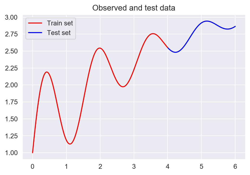
Simulated function we are interested in modelling with a GP. We will take samples from the red section and see how well the GP can recreate the blue section

class ExactGP(gpytorch.models.ExactGP):
    def __init__(self, train_x, train_y, likelihood):
        super(ExactGP, self).__init__(train_x, train_y, likelihood)
        self.mean_module = gpytorch.means.ConstantMean() # mean
        self.covar_module = gpytorch.kernels.ScaleKernel(gpytorch.kernels.RBFKernel()) # kernel

    def forward(self, x):
        mean_x = self.mean_module(x) 
        covar_x = self.covar_module(x) 
        return gpytorch.distributions.MultivariateNormal(mean_x, covar_x)

# initialize likelihood and model
likelihood = gpytorch.likelihoods.GaussianLikelihood()
model = ExactGP(train_x, train_y, likelihood)

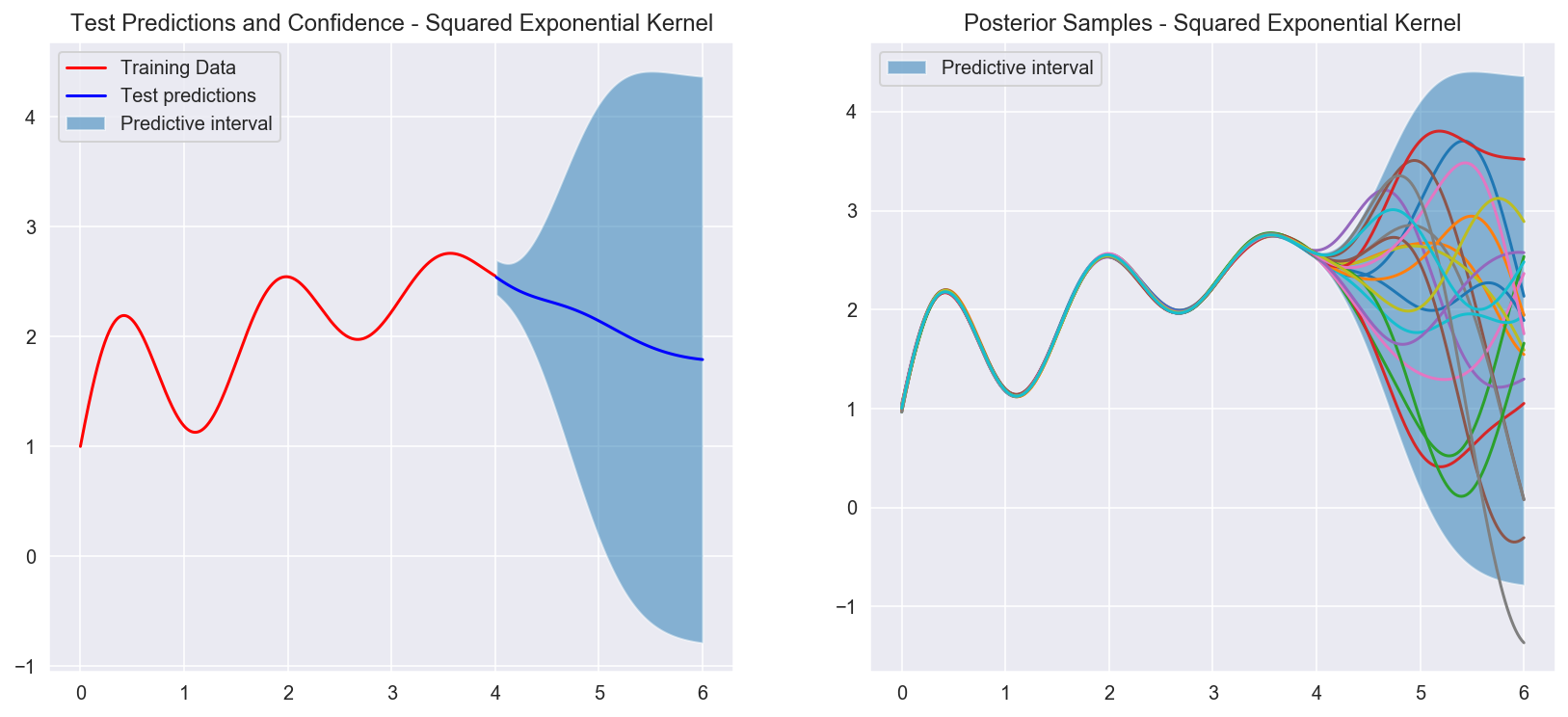
Posterior distribution after fitting the data in red. The graph on the left shows the confidence interval for the test set (blue region). As we get further and further away from the observed data, the confidence band grows. The graph on the right shows samples from the posterior distrubtion. Because we condition on the data and don't add noise, we are forcing the posterior to "pass through" every single one of our observed datapoints.