Hierarchical Models in Numpyro

In this post, I explore 3 different formulations for modelling repeated Bernoulli / binary trial data: complete pooling where all items have the same chance of success, no pooling where each item has an independent chance of success and partial pooling where data across items are shared to estimate parameters. To demonstrate, I model the free throw percentage of NBA players using Numpyro. Another famous example is modelling baseball batting averages, but I like basketball a lot more than baseball!

All the code for this post is available here.

In a repeated Bernoulli / binary trial, our data consists of $n$ units where each unit, $i$, records $y_i$ successes in $K_i$ trials / attempts. Two simple examples are in baseball and basketball, but they get a lot more interesting than this.

• Baseball batters: Every pitch faced is a trial and every hit is a success. Each batter is a unit.
• Basketball players taking free throws: Every free throw is a trial and every time they make it is a success. Each player is a unit

Problem and Data

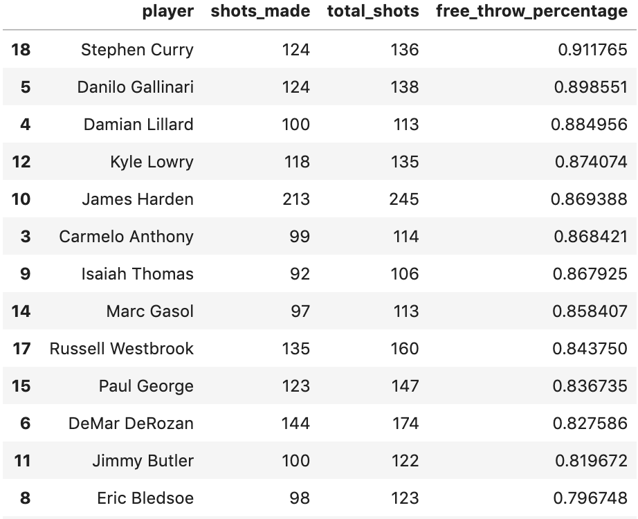
I’ll use NBA free throw data to model the free throw percentage of top players in the 2015-2016 season. To have a sort of train/test split, only the first quarter of the season will be used to fit the models and the other $\frac{3}{4}$ will be for testing / other stuff. Here’s what the data looks like after some manipulation:

Overall Model

The three formulations in this post branch out from the same canonical model. We have 16 players, $i = 1…16$, and our goal is to estimate the free throw percentage (chance of success) for each one, $\theta_i$. Our data consists of the number of shots made for player, $y_i$, and the number of attempts for each player, $K_i$. Using this, the number of free throws made, $y_i$, follows a Binomial distribution conditional on the number of attempts and probability of success:

To help with inference, we transform $\theta$ to a log-odds parameter, $\alpha$. Using $\alpha$ will change the distribution of $y_i$ from a Binomial distribution to a BinomialLogit, but the intuition is the same.

We are interested in estimating $\theta_i = \text{sigmoid}(\alpha_i)$, and our 3 formulations make different assumptions to do this.

Complete Pooling - Same $\theta$ for every player

In the complete pooling formulation, each player has the same chance of success parameter. This translates to each player having the same chance of making a free throw. The advantage of this is that we can aggregate all attempts and all successes for the players to “get” more data. However, this is a terrible assumption because we know some players are better at making free throws than others.

For this model, the likelihood and prior are below, notice that $\theta$ (and by extension, $\alpha$) is not indexed because there is only 1.

The prior on $\alpha$ can be interpreted as $95\%$ of values falling between a $0.26$ and $0.95$ chance of success.

def fully_pooled(ft_attempts, ft_makes=None):
    num_players = ft_attempts.shape[0]
    alpha = numpyro.sample("alpha", dist.Normal(1, 1)) # prior on \alpha
    theta = numpyro.deterministic("theta", jax.nn.sigmoid(alpha)) # need to use arviz
    with numpyro.plate("num_players", num_players):
        numpyro.sample("obs", dist.BinomialLogits(total_count = ft_attempts, logits=alpha), 
                       obs=ft_makes)

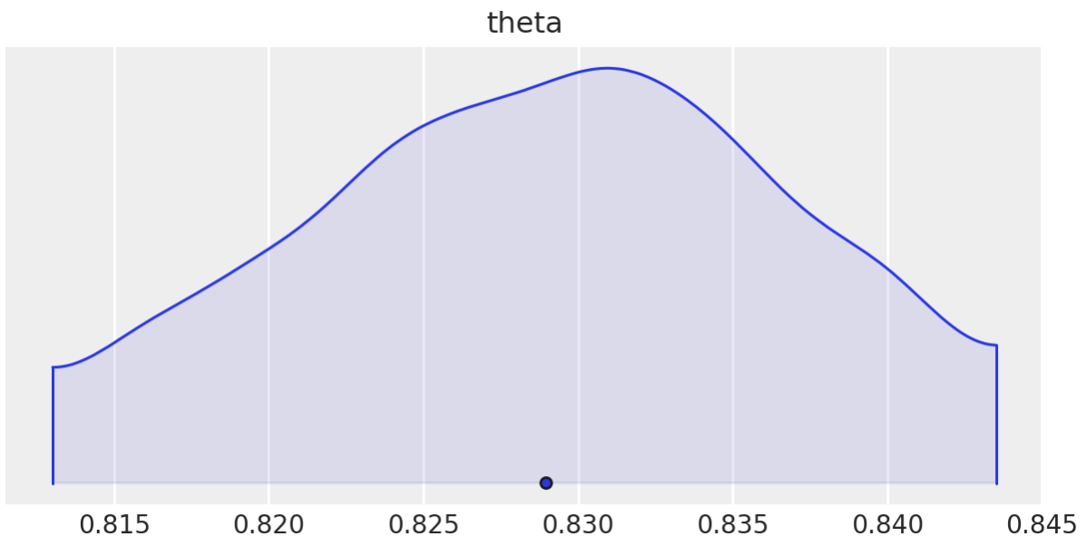
The posterior distribution for $\theta$ is below. Judging from the interval, we would be hard-pressed to find a player with a free throw percentage over $83.5\%$, however, $9$ out of the $16$ players analyzed have a free throw percentage higher than $83.5\%$. Aside from the assumptions of this model being completely wrong, it seems like the bi-product is a gross underestimation of players’ abilities. I guess this is expected since there will also be some overestimation for lower-ability players.

No Pooling - Independent $\theta_i$ for each player

The no pooling model is the exact opposite of the complete pooling model, where each player has a separate and independent chance of success. The formulation looks similar with a subtle difference, $\theta$ now becomes $\theta_i$ because there is a separate one for each player. Practically, this is exactly what we want as we know that each player has different free-throw abilities. However, we run into problems when we take into consideration the size of our dataset. We only have around 150 attempts for each player and have to use this to come up with a reliable estimate of ability. We’ll see the impact of this soon.

def no_pooling (ft_attempts, ft_makes = None):
    num_players = ft_attempts.shape[0]
    with numpyro.plate("players", num_players):
        alpha = numpyro.sample("alpha", dist.Normal(1, 1)) # prior
        assert alpha.shape == (num_players,), "alpha shape wrong" # one alpha for each player
        theta = numpyro.deterministic("theta", jax.nn.sigmoid(alpha))
        return numpyro.sample("obs", dist.BinomialLogits(total_count=ft_attempts, logits=alpha), 
                              obs = ft_makes) # likelihood

The posterior distributions for each $\theta$ are below:

It’s difficult to evaluate these estimates using only this graph, but one thing we can note is the size of the intervals. Many of them overlap significantly with a free throw percentage of $90\%$ and higher. This is an extremely high percentage, which is apparently close to getting you onto the top 50 all-time list. So it seems like the no-pooling formulation overestimates the player’s abilities.

Here is probably where I should note that I’m not particularly familiar with the difference between a good and great free throw percentage, but some Googling can go a long way.

Partial Pooling - Hierarchical Model

We ideally want a balance between the two extremes of no-pooling and complete-pooling, and this comes in the form of a partially pooled model. This model has a very subtle but important difference to the no pooling model which is in how we generate $\alpha_i$. Instead of sampling $\alpha_i$ directly from $N(1, 1)$, we estimate the mean, $\mu$, and standard deviation, $\sigma$, of $p(\alpha_i)$ using hyper-priors. Here, $\mu$ can be interpreted as the population chance of success. This difference may seem inconsequential but in small data settings, it makes the world of difference.

def partial_pooling (ft_attempts, ft_makes = None):
    num_players = ft_attempts.shape[0]
    mu = numpyro.sample("mu", dist.Normal(1, 1))
    sigma = numpyro.sample("sigma", dist.Normal(0, 1))
    with numpyro.plate("players", num_players):
        alpha = numpyro.sample("alpha", dist.Normal(mu, sigma))
        theta = numpyro.deterministic("theta", jax.nn.sigmoid(alpha))
        assert alpha.shape == (num_players, ), "alpha shape wrong"
        return numpyro.sample("y", dist.BinomialLogits(logits = alpha, total_count = ft_attempts), 
                              obs = ft_makes)

The plots below compare the posterior densities for the partial pooled and no-pooled models. The intervals from the partial pooled are narrower and seem better calibrated to what we expect to see in real life. Only three intervals overlap with $90\%$, and based on the players they seem reasonable.

While running these experiments, there was a noticeable difference in the posterior intervals when the amount of data is reduced. As the size of data was reduced, the hierarchical model became much more reliable than the no-pooling model.

Where does the difference come from?

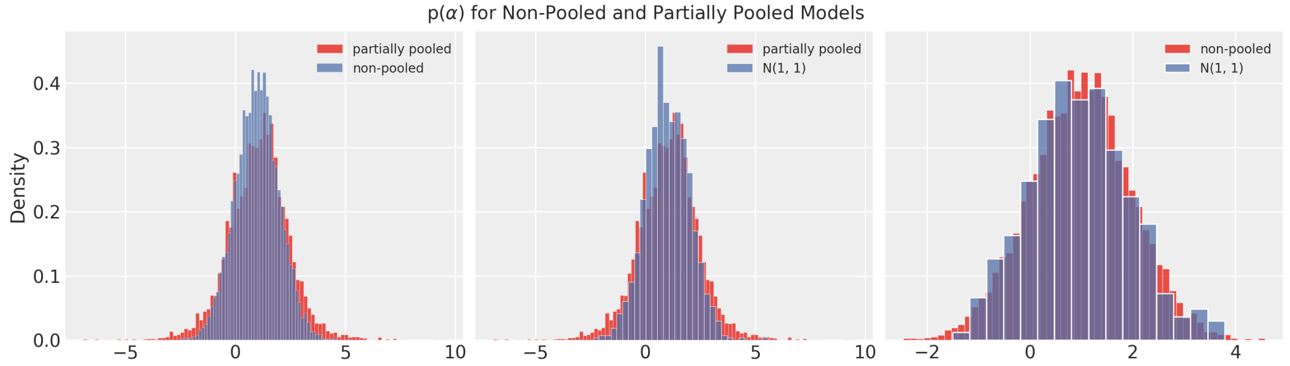
The partially pooled and non-pooled models have very similar formulations but produce very different posterior distributions. The most obvious difference in the formulation the prior on $\alpha_i$. The partial pooling formulation has more flexibility here as both $\mu$ an $\sigma$ are estimated from the data. Below I compare $p(\alpha)$ for the partially pooled and non-pooled models and it seems like the partially pooled prior has more variance than the non-pooled model.

I was interested to see the impact of flatter priors on the model. However, after increasing the prior variance for the non-pooled model, interval estimates were too wide to be useful, this is because we have such small data on each player. On the other hand, the interval estimates produced by the hierarchical model were very similar to before, this is because the hyper-priors are estimated using population data, which we have more of because of pooling. It turns out that as we collect more and more data, the no-pooling and partially pooled formulations converge to the same solutions.

Checking Model Interpretation

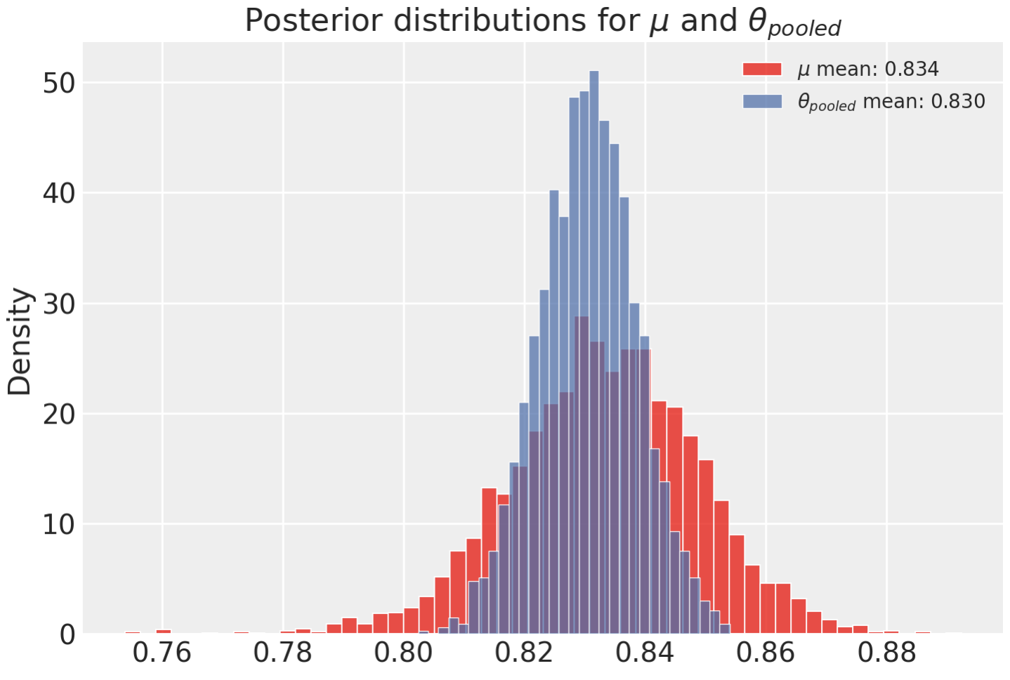
Above I mentioned that an interpretation of $\mu$ in the hierarchical model is the population chance of success. In our complete pooling formulation, $\theta$ is exactly the population chance of success. Here I compare the posterior distributions of these two parameters to see how similar they are. Before this is done, $\mu$ needs to be transformed from a log-odds parameter to a probability with $\text{sigmoid}(\mu)$.

Conclusion

There is a subtle but interesting difference between the no-pooling and partial pooling formulations that becomes more apparent as the data gets smaller. As we get more and more data, these two models converge to the same solutions.

Resources

• Hierarchical Partial Pooling for Repeated Binary Trials
• Numpyro with Arviz
• Bayesian hierarchical model for the prediction of football results