Introduction
In this post I build a Bayesian hierarchical model to classify Amazon products from Kaggle into a taxonomy using their titles. The taxonomy is hierarchical in nature and we can benefit from incorporating this structure into a model. First we’ll look at the taxonomy and class membership, then talk about simple approaches to the classification problem. Finally, we’ll build the Bayesian model and write it up in Numpyro.
Hierarchical Class Structure
Below is a diagram of the class structure. Each product (datapoint) is a member of a child category, which is in turn a member of a parent category. For example a broom is a member of the “household supplies” child category, which is in turn a member of the “health personal care” parent category. For this problem we have $6$ parent classes and $64$ child classes.
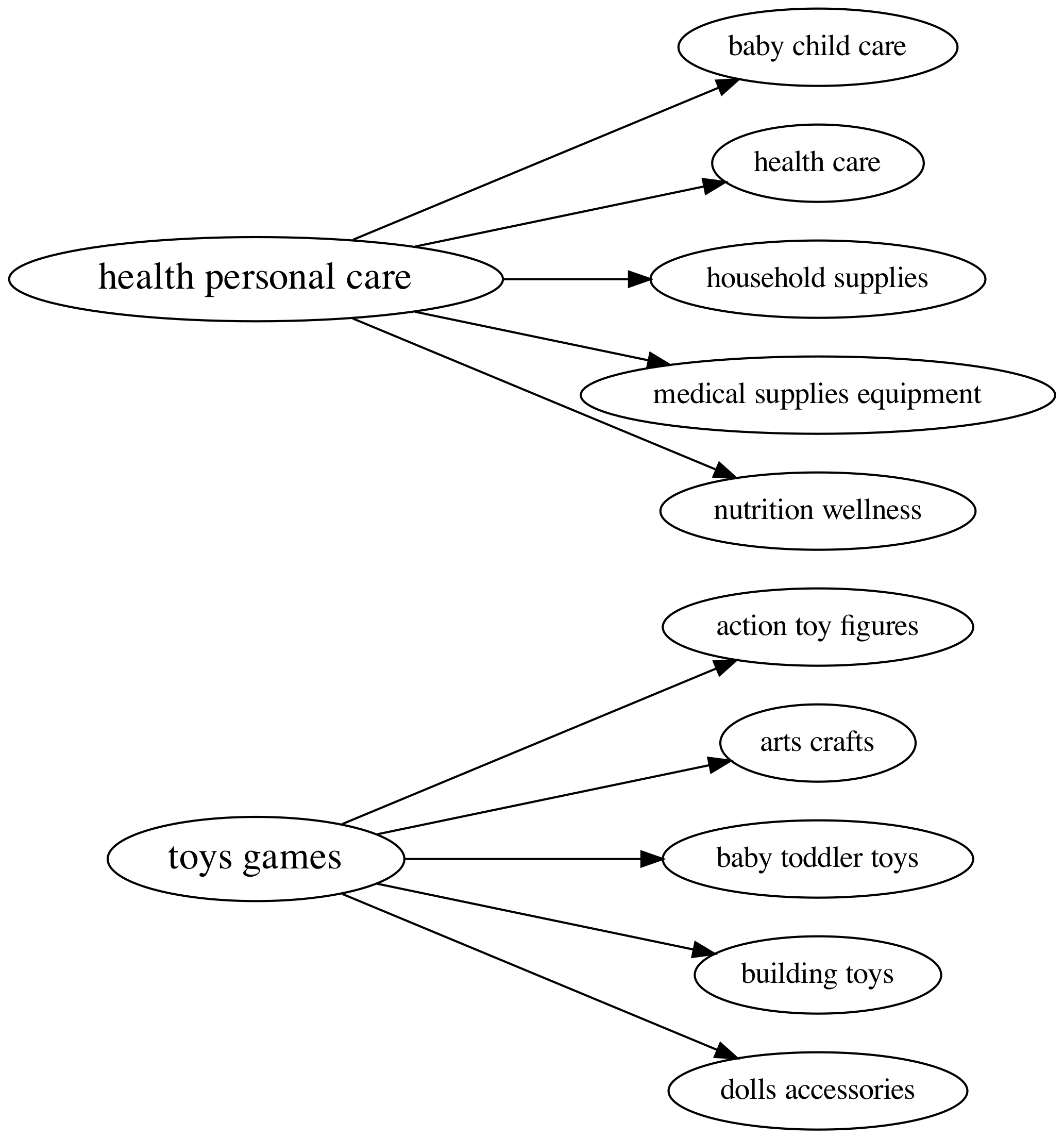
Taxonomy structure for 2 parent classes (on the left) and 5 of their children classes (on the right). This is a small subset of parent and children classes.
A simple way of assigning categories to our data would be to flatten the hierarchy and only consider the child classes. This would turn our problem into a $64$ class classification problem which can be solved with logistic regression / SVM / many other things. The drawback of this approach is that we make the assumption that each class is independednt, which we know is incorrect.
We want to leverage the fact that “action toy figures” and “baby toddler toys” come from the same parent class, “toy games”. Intuitively, this can help when we don’t have a lot of training data for a particular child class, or if we come across an item at inference time that we don’t have a subclass for. One way to deal with this problem is by using hierarchical modelling.
Data and Preprocessing
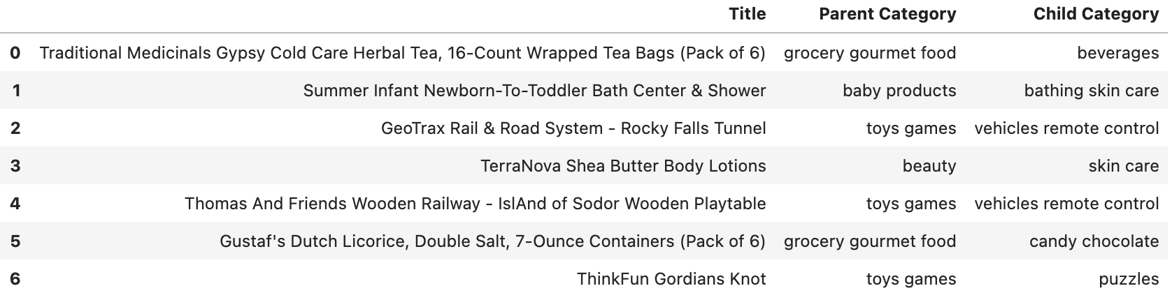
Before diving into the model, here is the data we’re working with:
I use TF-IDF scores of item titles to classify them into the taxonomy. Gensim was used to calculate TF-IDF scores, but sklearn is fine. I found that Gensim is more memory efficient when working with much larger datasets.
%%time
# find tf-idf scores for training set
dct = Dictionary(X_train.map(lambda x: x.split(' ')))
dct.filter_extremes(no_below=5, no_above=0.7, keep_n = 2 ** 5)
dct.compactify()

train_corpus = [dct.doc2bow(doc.split(' ')) for doc in X_train]  # BoW format
tfidf_model = TfIdfTransformer()

train_tfidf = tfidf_model.fit_transform(train_corpus)
train_tfidf = corpus2dense(train_tfidf, num_terms = len(dct)) # can also use: corpus2csc
print(train_tfidf.shape)

test_corpus = [dct.doc2bow(doc.split(' ')) for doc in X_test]
test_tfidf = corpus2dense(tfidf_model.transform(test_corpus), num_terms = len(dct))
print(test_tfidf.shape)
Finally we encode the labels for parent and children classes in 2 different ways: labelEncoder and labelBinarizer. The former maps each class into an integer, which we’ll use to fit a couple sklearn models to compare against our Bayesian model. The latter one-hot encodes the target variable, which we’ll use for the Bayesian model.
le = preprocessing.LabelEncoder()
parent_target = le.fit_transform(parent_train)
children_target = le.fit_transform(children_train)

parent_target_test = le.fit_transform(parent_test)
children_target_test = le.fit_transform(children_test)

lb = LabelBinarizer()
parent_binr = lb.fit_transform(parent_train)
children_binr = lb.fit_transform(children_train)
Bayesian Hierarchical Modeling
The class structure can be explicitly represented by our priors in a hierarchical model, so let’s do that. Our underlying model will be a logistic regression with target, $y$, being the children classes. Therefore $\beta \in R^{p \times c}$, where $p$ is the length of the TF-IDF vector and $c$ is the number of children classes, $64$ in this case.
\[Z = X \beta + \epsilon\] \[y = \text{softmax}(Z)\]Column $i$ of $\beta$ are the regression coefficients for class $i$. We know that class $i$ is the child of parent class $p_i$, and that $i$ has siblings which also come from parent class $p_i$. We want each child of parent $p_i$ to have the same prior, which we can represent below:
\[\begin{equation*} \beta_p \sim N(\beta_{\mu_p}, \sigma_{\mu_p}^2) \\[10pt] \beta_c = \beta_p \times \alpha \\[10pt] \beta \sim N(\beta_c, \sigma_c^2) \\[10pt] \epsilon \sim N(0, 1) \\[10pt] \end{equation*}\]Here, $\beta_{\p}$ is the hierarchical prior for each parent class and $\beta_c$ is the prior mean for each child class. We transform $\beta_p$ into $\beta_c$ by multiplying by another matrix, $\alpha \in R^{p \times c}$. This $\alpha$ is a matrix that links each children class to its parent.
Inference in Numpyro
Numpyro is another probabilistic programming language built on Pyro and JAX. It’s supposed to blazing fast thanks to speed ups provided by JAX, so this is a good opportunity to try it out.
# functions for inference and prediction. Will post the model code soon.
# helper function for HMC inference
def run_inference(model, rng_key, X, Y,
                  num_warmup = 10,
                  num_samples = 100,
                  num_chains = 2):
    start = time.time()
    kernel = NUTS(model)
    print("Starting MCMC: ")
    mcmc = MCMC(kernel, num_warmup = num_warmup,
                num_samples = num_samples,
                num_chains = num_chains)
    mcmc.run(rng_key, X, Y)
    print('\nMCMC elapsed time:', time.time() - start)
    return mcmc

# helper function for prediction
def predict(model, rng_key, samples, X):
    model = handlers.substitute(handlers.seed(model, rng_key), samples)
    # note that Y will be sampled in the model because we pass Y=None here
    model_trace = handlers.trace(model).get_trace(X=X, Y=None)
    return model_trace['Y']['value']
Numpyro provides a reparam function, to change hierarchical model specifications from centered to non-centered parameterizations. We’ll use this to help with inference.
X = jnp.asarray(train_tfidf.T, dtype = "float32")
Y = jnp.asarray(children_binr, dtype = "float32") # binarized labels

_num_chains = 4
_num_samples = 200
numpyro.set_host_device_count(_num_chains)
rng_key, rng_key_predict = random.split(random.PRNGKey(0))

reparam_model = reparam(hierarchical_model, config={'beta': LocScaleReparam(0)})
non_centered_mcmc = run_inference(model = reparam_model,
                                  rng_key = rng_key,
                                  X = X, Y = Y,
                                  num_warmup = 50,
                                  num_samples = _num_samples,
                                  num_chains = _num_chains,
                                  chain_method = 'vectorized')
nc_samples = non_centered_mcmc.get_samples()

print("MCMC complete")
Train set accuracy, child categories:  0.7351668726823238
Test set accuracy, child categories:  0.6277708071936429
Comparison to Flat Classification
Of course, we need to compare this hierarchical model against simpler formulations. One of the simplest approaches to this problem is to flatten the hierarchy, which we do by disregarding the parent classes. We’ll compare a Ridge classifier, SVM classifier and logistic regression:
# rige classifier
ridge_clf = RidgeClassifier().fit(train_tfidf.T, children_target)
print("Ridge classifier train set accuracy, children classes: ", ridge_clf.score(train_tfidf.T, children_target))
print("Ridge classifier test set accuracy, children classes: ", ridge_clf.score(test_tfidf.T, children_target_test))

print('')

# linear SVM
sgd_clf = SGDClassifier(loss = "hinge", # linear SVM, "log" for logistic regression
                        max_iter=1000,
                        n_jobs = -1,
                        random_state = 42,
                        tol=1e-3).fit(train_tfidf.T, children_target)
print("SVM classifier train set accuracy, children classes: ", sgd_clf.score(train_tfidf.T, children_target))
print("SVM classifier test set accuracy, children classes: ", sgd_clf.score(test_tfidf.T, children_target_test))

print('')

# logistic regression
log_reg = SGDClassifier(loss = "log", # linear SVM, "log" for logistic regression
                        max_iter=1000,
                        n_jobs = -1,
                        random_state = 42,
                        tol=1e-3).fit(train_tfidf.T, children_target)
# log_reg.predict_proba(test_tfidf.T)
print("Logistic Regression train set accuracy, children classes: ", log_reg.score(train_tfidf.T, children_target))
print("Logistic Regression test set accuracy, children classes: ", log_reg.score(test_tfidf.T, children_target_test))
Ridge classifier train set accuracy, children classes:  0.7184796044499382
Ridge classifier test set accuracy, children classes:  0.6273525721455459

SVM classifier train set accuracy, children classes:  0.7481458590852905
SVM classifier test set accuracy, children classes:  0.6288163948138854

Logistic Regression train set accuracy, children classes:  0.7081788215904409
Logistic Regression test set accuracy, children classes:  0.6286072772898369
Next Steps
There is where this post stops because of time constraints, but to really understand the differences in models, I’m writing some interesting areas to look into in the future.
- Performance of parent categories: I expect the hierarchical model to perform well on the parent-level categories, since we implicitly model these in our regression. In particular I’m interested in the parent-level preformance for classes that have few datapoints.
- Out-of-distribution examples: Because our model is Bayesian, it should also be able to detect out-of-distribution samples better than the frequentist models. We can test this by applying a random text dataset to the models.
Bloopers: Parent Posterior as Children Prior
I also experimented with another formulation where I first fit a logistic regression to predict the parent classes, and obtained the posterior mean for $\beta_p$. I then used $\beta_p$ as the prior mean for another regression, where I predict the children classes. Th formulation turned out to not work as well as the traditional hierarchical model, and I suspect it is because when using the posterior mean of $\beta_p$, the posterior variance was disregarded. This no longer made the model hierarchical, but simply just changed the prior mean for $\beta_c$.
The code I used to run this is below:
# first fit parent regression
def parent_model(X, Y=None):
    if Y == None :
        dim_Y = 6
    else :
        dim_Y = Y.shape[1]
    beta = numpyro.sample("beta", dist.Normal(jnp.zeros((X.shape[1], dim_Y)), jnp.ones((X.shape[1], dim_Y))*2))
    err = numpyro.sample("err", dist.Normal(0., 1.))
    resp = jnp.matmul(X, beta) + err
    probs = softmax(resp) # jax softmax, not scipy
    numpyro.sample("Y", dist.Multinomial(probs = probs), obs = Y)


X = jnp.asarray(train_tfidf.T, dtype = "float32")
Y = jnp.asarray(parent_binr, dtype = "float32") # binarized labels

_num_chains = 4
_num_samples = 200
numpyro.set_host_device_count(_num_chains)
rng_key, rng_key_predict = random.split(random.PRNGKey(0))
mcmc = run_inference(model = parent_model,
                     rng_key = rng_key,
                     X = X, Y = Y,
                     num_warmup = 50,
                     num_samples = _num_samples,
                     num_chains = _num_chains)
parent_samples = mcmc.get_samples()
print("MCMC complete")

# predict Y_test at inputs X_test
vmap_args = (parent_samples, random.split(rng_key_predict, _num_chains * _num_samples))
predictions = vmap(lambda samples, rng_key: predict(parent_model, rng_key, samples, X))(*vmap_args)

# compute mean prediction and confidence interval around median
mean_prediction = jnp.mean(predictions, axis=0)
percentiles = np.percentile(predictions, [5.0, 95.0], axis=0)

class_predictions = pd.DataFrame(mean_prediction).apply(np.argmax, axis = 1)
print("Training set accuracy: ", np.mean(class_predictions == parent_target))
Now construct the prior mean for the child regression by using the posterior mean of the parent regression.
# use the posterior of the parent regression as the prior mean for the child regression
beta_posterior = parent_samples["beta"]
posterior_mean = np.apply_along_axis(np.mean, 0, beta_posterior)

posterior_mean_df = pd.DataFrame(posterior_mean, columns = parent_class_list)

prior_mean = pd.DataFrame()
for c in children_class_list :
    prior_mean[c] = posterior_mean_df[class_tree[c]]

prior_mean.head()
And re-run a similar model, but this time using the children labels as the target:
# model for the child classes
def child_model(X, Y=None):
    beta = numpyro.sample("beta", dist.Normal(jnp_prior_mean, jnp.ones(jnp_prior_mean.shape)*2))
    err = numpyro.sample("err", dist.Normal(0., 0.5))
    resp = jnp.matmul(X, beta) + err
    probs = softmax(resp) # jax softmax, not scipy
    numpyro.sample("Y", dist.Multinomial(probs = probs), obs = Y)

X = jnp.asarray(train_tfidf.T, dtype = "float32")
Y = jnp.asarray(children_binr, dtype = "float32") # binarized labels
jnp_prior_mean = jnp.asarray(prior_mean, dtype = "float32")

_num_chains = 4
_num_samples = 500
numpyro.set_host_device_count(_num_chains)
rng_key, rng_key_predict = random.split(random.PRNGKey(0))

child_model_reparam = reparam(child_model, config={'beta': LocScaleReparam(0)})

child_mcmc = run_inference(model = child_model_reparam,
                           rng_key = rng_key,
                           X = X, Y = Y,
                           num_warmup = 50,
                           num_samples = _num_samples,
                           num_chains = _num_chains)
child_samples = child_mcmc.get_samples()
print("MCMC complete")


# predict Y_test at inputs X_test
vmap_args = (child_samples, random.split(rng_key_predict, _num_chains * _num_samples))
children_predictions = vmap(lambda samples, rng_key: predict(child_model, rng_key, samples, X))(*vmap_args)

# compute mean prediction and confidence interval around median
mean_children_prediction = jnp.mean(children_predictions, axis=0)
percentiles = np.percentile(children_predictions, [5.0, 95.0], axis=0)

child_class_predictions = pd.DataFrame(mean_children_prediction).apply(np.argmax, axis = 1)
print("Train set accuracy, child categories: ", np.mean(child_class_predictions == children_target))
The test set accuracy of the child model using this formulation was around 44%, significantly worse than both the frequentist models and non-centered hierarchical model.